Merton Model Calibration
We will look at how to use previously learned methods like Lewis (2001) on Merton (1976) model in order to perform model calibration. As was the case in the previous module, most of the code in this blog is based on and adapted from Hilpisch’s Derivatives Analytics with Python.
To start with, let’s import the necessary libraries:
import matplotlib.pyplot as plt
import numpy as np
from scipy.integrate import quad
1. Lewis (2001) Approach
Let’s start by revisiting the Fourier methods for pricing in the Merton (1976) model. Essentially, under the Lewis (2001) approach, the value of the Call option is determined by: \(\begin{equation*} C_0 = S_0 - \frac{\sqrt{S_0 K} e^{-rT}}{\pi} \int_{0}^{\infty} \mathbf{Re}[e^{izk} \varphi(z-i/2)] \frac{dz}{z^2+1/4} \end{equation*}\) which means that we just need the characteristic function of the process in Merton (1976).
1.1. Merton (1976) Characteristic Function
Merton’s (1976) characteristic function is given by: \(\begin{equation*} \varphi^{M76}_0 (u, T) = e^{\left( \left( i u \omega - \frac{u^2 \sigma^2}{2}+ \lambda ( e^{i u \mu_j - u^2 \delta^2/2}-1) \right) T \right)} \end{equation*}\) where, \(\begin{equation*} \omega = r - \frac{\sigma^2}{2} - \lambda \left( e^{\mu_j + \delta^2/2}-1 \right) \end{equation*}\) Thus, let’s start by coding this characteristic function:
def M76_char_func(u, T, r, sigma, lamb, mu, delta):
"""
Characteristic function for Merton '76 model
"""
omega = r - 0.5 * sigma**2 - lamb * (np.exp(mu + 0.5 * delta**2) - 1)
char_func_value = np.exp(
(
1j * u * omega
- 0.5 * u**2 * sigma**2
+ lamb * (np.exp(1j * u * mu - u**2 * delta**2 * 0.5) - 1)
)
* T
)
return char_func_value
1.2. Lewis (2001) Integral Value
The next step is to define the value of the integral in Lewis (2001) given the characteristic function:
def M76_integration_function(u, S0, K, T, r, sigma, lamb, mu, delta):
"""
Integral function for Lewis (2001) under Merton'76 characteristic function
"""
char_func = M76_char_func(u - 0.5 * 1j, T, r, sigma, lamb, mu, delta)
value = 1 / (u**2 + 0.25) * (np.exp(1j * u * np.log(S0 / K)) * char_func).real
return value
And the value of the Call option:
def M76_call_value(S0, K, T, r, sigma, lamb, mu, delta):
"""
Value of the Call option under Lewis (2001) for Merton'76 jump diffusion model
"""
int_value = quad(
lambda u: M76_integration_function(u, S0, K, T, r, sigma, lamb, mu, delta),
0,
50,
limit=250,
)[0]
call_value = max(0, S0 - np.exp(-r * T) * np.sqrt(S0 * K) / np.pi * int_value)
return call_value
1.3. Pricing Example with Given Parameters
Once we have this set of functions, we can, given some parameters, price a call option under the Merton (1976) jump diffusion model. For example, assume the following parameters:
- $S_0 = 100$
- $K = 100$
- $T=1$
- $r = 0.05$
- $\sigma = 0.4$
- $\lambda = 1.0$
- $\mu = -0.2$
- $\delta = 0.1$ What would be the price of a Call option under Lewis (2001)?
S0 = 100
K = 100
T = 1
r = 0.05
sigma = 0.4
lamb = 1
mu = -0.2
delta = 0.1
print(
    "Value of the Call option under Merton (1976) is:  $",
    M76_call_value(S0, K, T, r, sigma, lamb, mu, delta),
)
Value of the Call option under Merton (1976) is:  $ 19.947853881446505
2. Merton (1976) Model Calibration
The next step is to calibrate the Merton (1976) model to observed option market prices in order to infer the model parameters. In order to do so, we are going to follow a very similar approach to that of the Heston model developed in the past module. In fact, we are going to use the same option market data file from the previous module on EuroStoxx 50 options.
2.1. Obtaining Options Market Data
import pandas as pd
from scipy.optimize import brute, fmin
# Market Data from www.eurexchange.com
# as of September 30, 2014
h5 = pd.HDFStore(
"option_data_M2.h5", "r"
) # Place this file in the same directory before running the code
data = h5["data"] # European call & put option data (3 maturities)
h5.close()
S0 = 3225.93 # EURO STOXX 50 level September 30, 2014
As was the case in the previous post, we will select near ATM options:
# Option Selection
tol = 0.02 # Tolerance level to select ATM options (percent around ITM/OTM options)
options = data[(np.abs(data["Strike"] - S0) / S0) < tol]
options["Date"] = pd.DatetimeIndex(options["Date"])
options["Maturity"] = pd.DatetimeIndex(options["Maturity"])
Then, we add time left until maturity and a constant risk-free rate:
# Adding Time-to-Maturity and constant short-rates
for row, option in options.iterrows():
T = (option["Maturity"] - option["Date"]).days / 365.0
options.loc[row, "T"] = T
options.loc[row, "r"] = 0.005 # ECB base rate
options.head()
Date Strike Call Maturity Put T r
38 2014-09-30 3175.0 126.8 2014-12-19 78.8 0.219178 0.005
39 2014-09-30 3200.0 110.9 2014-12-19 87.9 0.219178 0.005
40 2014-09-30 3225.0 96.1 2014-12-19 98.1 0.219178 0.005
41 2014-09-30 3250.0 82.3 2014-12-19 109.3 0.219178 0.005
42 2014-09-30 3275.0 69.6 2014-12-19 121.6 0.219178 0.005
2.2. Defining Error Functions
Once we have options market data that we have to “match” with our model, our next step is to define an error function for the specific case of the Merton model. In this case, we will use the Root Mean Squared Error (RMSE) as a measure. This is basically defined as: \begin{equation} RMSE = \sqrt{\frac{1}{N}\sum_{n=1}^N \left( C^_n - C^{M76}_n\right)^2} \end{equation} where $C^$ is observed market prices and $C^{M76}$ are the values produced by Merton’s (1976) model.
i = 0
min_RMSE = 100
def M76_error_function(p0):
"""
Error function for parameter calibration in Merton'76 model
---------------
Parameters to calibrate:
sigma: float
volatility factor in diffusion term
lambda: float
jump intensity
mu: float
expected jump size
delta: float
standard deviation of jump
----------------
RMSE: Root Mean Squared Error
"""
global i, min_RMSE
sigma, lamb, mu, delta = p0
if sigma < 0.0 or delta < 0.0 or lamb < 0.0:
return 500.0
se = []
for row, option in options.iterrows():
model_value = M76_call_value(
S0, option["Strike"], option["T"], option["r"], sigma, lamb, mu, delta
)
se.append((model_value - option["Call"]) ** 2)
RMSE = np.sqrt(sum(se) / len(se))
min_RMSE = min(min_RMSE, RMSE)
if i % 50 == 0:
print("%4d |" % i, np.array(p0), "| %7.3f | %7.3f" % (RMSE, min_RMSE))
i += 1
return RMSE
2.3. Calibration Function
Next, we need to create our calibration function. This follows the same logic as in the case of Heston from the previous module. For illustrative purposes, let’s set a somewhat high tolerance level so that the optimization does not convey time. By the end of this blog, we will dig deeper into the different issues that arise when accurately calibrating a model.
def M76_calibration_full():
"""
Calibrates Merton (1976) stochastic volatility model to market quotes
"""
# First run with brute force
# (scan sensible regions, for faster convergence)
p0 = brute(
M76_error_function,
(
(0.075, 0.201, 0.025), # sigma
(0.10, 0.401, 0.1), # lambda
(-0.5, 0.01, 0.1), # mu
(0.10, 0.301, 0.1),
), # delta
finish=None,
)
# Second run with local, convex minimization
# (we dig deeper where promising results)
opt = fmin(
M76_error_function, p0, xtol=0.0001, ftol=0.0001, maxiter=550, maxfun=1050
)
return opt
opt = M76_calibration_full()
0 | [ 0.075 0.1 -0.5 0.1 ] | 31.540 | 31.540
50 | [ 0.075 0.3 -0.1 0.3 ] | 22.852 | 11.298
100 | [ 0.1 0.2 -0.2 0.2] | 19.922 | 8.654
150 | [ 0.125 0.1 -0.3 0.1 ] | 10.704 | 5.571
200 | [ 0.125 0.4 -0.5 0.3 ] | 55.500 | 4.662
250 | [0.15 0.2 0. 0.2 ] | 6.619 | 3.586
300 | [ 0.175 0.1 -0.1 0.1 ] | 14.171 | 3.586
350 | [ 0.175 0.4 -0.3 0.3 ] | 54.376 | 3.586
400 | [ 0.2 0.3 -0.4 0.2] | 63.380 | 3.586
450 | [ 0.14702168 0.19533978 -0.10189428 0.10218084] | 3.495 | 3.428
500 | [ 0.14987758 0.11503181 -0.14398098 0.09850597] | 3.401 | 3.401
550 | [ 0.15597729 0.01124105 -0.20255149 0.07785796] | 3.359 | 3.359
600 | [ 0.15617567 0.00947711 -0.20364524 0.07721602] | 3.358 | 3.358
Optimization terminated successfully.
Current function value: 3.358419
Iterations: 107
Function evaluations: 183
2.4. Plotting Results of Calibration
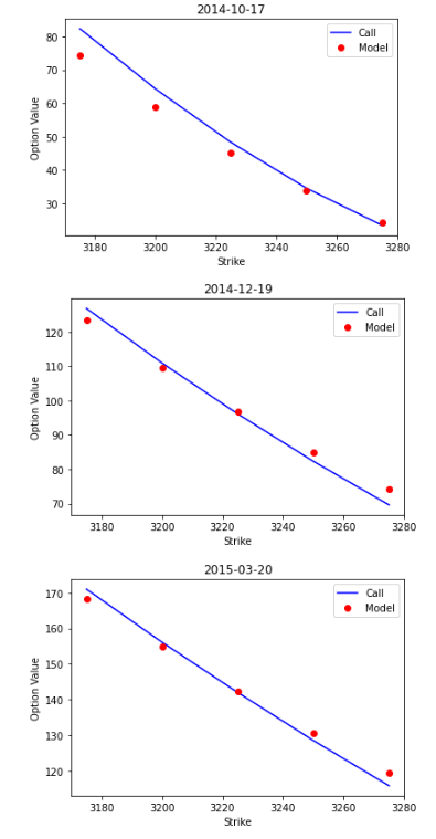
Finally, let’s see how our model calibration performs graphically. For this, we will create a function that plots the different estimates together with the observed market prices. Given that our dataset has option market prices for 3 different maturities, we will also check the performance of the calibration for the different maturities:
def generate_plot(opt, options):
# First, we calculate model prices
sigma, lamb, mu, delta = opt
options["Model"] = 0.0
for row, option in options.iterrows():
options.loc[row, "Model"] = M76_call_value(
S0, option["Strike"], option["T"], option["r"], sigma, lamb, mu, delta
)
# Second, we plot
mats = sorted(set(options["Maturity"]))
options = options.set_index("Strike")
for i, mat in enumerate(mats):
options[options["Maturity"] == mat][["Call", "Model"]].plot(
style=["b-", "ro"], title="%s" % str(mat)[:10]
)
plt.ylabel("Option Value")
generate_plot(opt, options)
3. Conclusion
This is all regarding Merton (1976) model calibration. We have basically repeated the process of the last module with Heston (1993) and adapted things to the Merton jump diffusion model. Now that you know how to properly calibrate somewhat simple models, we are going to make a step forward and look at a more complex one. Ideally, a model would incorporate stochastic volatility features present in Heston (1993), with the jump diffusion of Merton (1976). The question is, can we build a model that incorporates both of these desirable characteristics? The answer is yes, and that’s what we will begin to explore in the next post. References
- Hilpisch, Yves. Derivatives Analytics with Python: Data Analysis, Models, Simulation, Calibration and Hedging. John Wiley & Sons, 2015.