Stochastic Volatility: Heston
Introduction
We start dealing with stochastic volatility models. Specifically, we will implement the Monte-Carlo simulation of the Heston (1993) stochastic volatility model.
The Heston Stochastic Volatility Model is a mathematical model that aims to capture the evolution of an asset’s price and its associated volatility over time. Unlike the Black-Scholes model, which assumes constant volatility, the Heston model allows for time-varying volatility by modeling it as a stochastic process. This makes it a more flexible and realistic tool for option pricing and risk management.
Formula
The Heston model describes two stochastic differential equations (SDEs):
- For the asset price $ S(t) $:
- For the volatility $ V(t) $:
Where:
- $ \mu $ = Risk-free rate
- $ S(t) $ = Asset price at time $ t $
- $ V(t) $ = Volatility at time $ t $
- $ dW_1(t), dW_2(t) $ = Wiener processes, potentially correlated with correlation coefficient $ \rho $
- $ \kappa $ = Rate at which $ V(t) $ reverts to $ \theta $
- $ \theta $ = Long-term mean of the volatility process
- $ \xi $ = Volatility of volatility
Key Concepts
-
Stochastic Volatility: Unlike constant volatility models like Black-Scholes, the Heston model allows volatility to be a random function of time.
-
Mean Reversion: The model includes a mean-reversion term ($ \kappa (\theta - V(t)) $), which makes the volatility revert to a long-term mean ($ \theta $) over time.
-
Volatility of Volatility: The Heston model accounts for the “volatility of volatility” through the $ \xi $ term, allowing the model to capture the “smile” or “skew” in the implied volatility surface.
-
Correlation: The model also includes a term ($ \rho $) to capture the correlation between the asset price and its volatility.
To simulate these continuous-time processes, you often need to discretize them. This is done to approximate the changes in the asset price and volatility over small periods of time. A common method of discretization is the Euler-Maruyama scheme.
Discretization Using Euler-Maruyama Scheme
Euler-Maruyama is a numerical method used for approximating solutions to SDEs. In this scheme, a continuous-time stochastic process is approximated over discrete time intervals of length $ dt $. The scheme transforms the original continuous-time SDEs into the discrete-time formulas you presented.
Asset Price $ S_t $
\[S_t = S_{t-1} e^{\left( r - \frac{\nu_t}{2} \right) dt + \sqrt{\nu_t} dZ_1 \sqrt{dt}}\]Here, $ r $ is the risk-free rate, $ \nu_t $ is the volatility at time $ t $, $ dt $ is the time step, and $ dZ_1 $ is a sample from a standard normal distribution. The term $ e^{\left( r - \frac{\nu_t}{2} \right) dt} $ is the drift term, and $ \sqrt{\nu_t} dZ_1 \sqrt{dt} $ is the stochastic term.
Volatility $ \nu_t $
\[\nu_t = \nu_{t-1} + \kappa \left( \theta - \nu_{t-1} \right) dt + \xi \sqrt{\nu_{t-1}} dZ_2 \sqrt{dt}\]Here, $ \kappa $ is the rate at which volatility reverts to the long-term mean $ \theta $, $ \xi $ is the volatility of volatility, and $ dZ_2 $ is another sample from a standard normal distribution.
These formulas allow you to simulate $ S_t $ and $ \nu_t $ iteratively over a sequence of discrete time steps, thus providing a numerical approximation to the Heston model’s continuous-time behavior.
As usual, let’s start by importing the necessary libraries.
import matplotlib.pyplot as plt
import numpy as np
import scipy.stats as ss
We will start by coding the stochastic volatility function, 𝜈𝑡:
def SDE_vol(v0, kappa, theta, sigma, T, M, Ite, rand, row, cho_matrix):
    dt = T / M  # T = maturity, M = number of time steps
    v = np.zeros((M + 1, Ite), dtype=np.float)
    v[0] = v0
    sdt = np.sqrt(dt)  # Sqrt of dt
    for t in range(1, M + 1):
        ran = np.dot(cho_matrix, rand[:, t])
        v[t] = np.maximum(
            0,
            v[t - 1]
            + kappa * (theta - v[t - 1]) * dt
            + np.sqrt(v[t - 1]) * sigma * ran[row] * sdt,
        )
    return v
Next, let’s implement the classic stochastic equation for the underlying asset price evolution:
def Heston_paths(S0, r, v, row, cho_matrix):
    S = np.zeros((M + 1, Ite), dtype=float)
    S[0] = S0
    sdt = np.sqrt(dt)
    for t in range(1, M + 1, 1):
        ran = np.dot(cho_matrix, rand[:, t])
        S[t] = S[t - 1] * np.exp((r - 0.5 * v[t]) * dt + np.sqrt(v[t]) * ran[row] * sdt)

    return S
The last function we will define, just for simplifying the tasks, will be a random number generator following a standard normal:
def random_number_gen(M, Ite):
    rand = np.random.standard_normal((2, M + 1, Ite))
    return rand
Now that we have defined the main functions to use in the process, let’s implement the Heston model under some parameters (assume these are given for now):
v0 = 0.04
kappa_v = 2
sigma_v = 0.3
theta_v = 0.04
rho = -0.9

S0 = 100  # Current underlying asset price
r = 0.05  # Risk-free rate
M0 = 50  # Number of time steps in a year
T = 1  # Number of years
M = int(M0 * T)  # Total time steps
Ite = 10000  # Number of simulations
dt = T / M  # Length of time step
Finally, let’s work on the random number generator and the covariance matrix (using Cholesky decomposition to account for correlation between $dZ_1$ and $dZ_2$):
# Generating random numbers from standard normal
rand = random_number_gen(M, Ite)

# Covariance Matrix
covariance_matrix = np.zeros((2, 2), dtype=np.float)
covariance_matrix[0] = [1.0, rho]
covariance_matrix[1] = [rho, 1.0]
cho_matrix = np.linalg.cholesky(covariance_matrix)
Now we have all the ingredients to generate the paths for both asset price and its volatility:
# Volatility process paths
V = SDE_vol(v0, kappa_v, theta_v, sigma_v, T, M, Ite, rand, 1, cho_matrix)

# Underlying price process paths
S = Heston_paths(S0, r, V, 0, cho_matrix)
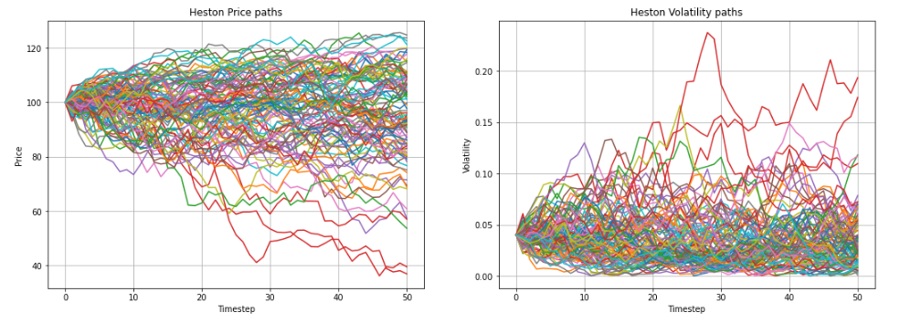
Let’s visualize some of the paths for both the underlying price and the volatility:
def plot_paths(n):
    fig = plt.figure(figsize=(18, 6))
    ax1 = fig.add_subplot(121)
    ax2 = fig.add_subplot(122)

    ax1.plot(range(len(S)), S[:, :n])
    ax1.grid()
    ax1.set_title("Heston Price paths")
    ax1.set_ylabel("Price")
    ax1.set_xlabel("Timestep")

    ax2.plot(range(len(V)), V[:, :n])
    ax2.grid()
    ax2.set_title("Heston Volatility paths")
    ax2.set_ylabel("Volatility")
    ax2.set_xlabel("Timestep")

plot_paths(100)
Statistical Distribution Produced by Heston
One important feature of the Heston model is that it produces a distribution of returns that has heavier tails and kurtosis than a normal distribution, just as we observe in practice.
In the following code snippet, we will check the Heston-produced distribution on two fronts:
-
Whether underlying returns resemble a Normal distribution, as assumed in BS and GBM process.
-
How volatility fits a mean-reverting process such as CIR or Vasicek.
# Obtaining degrees of freedom (do not worry a lot about this now)
c = 2 * kappa_v / ((1 - np.exp(-kappa_v * T)) * sigma_v**2)
df = 4 * kappa_v * theta_v / sigma_v**2
nc = 2 * c * v0 * np.exp(-kappa_v * T)


# Calculating returns and lengths of axis
log_R = np.log(S[-1, :] / S0)
x = np.linspace(log_R.min(), log_R.max(), 500)
y = np.linspace(0.00001, 0.1, 500)


# Plotting the different distributions
fig = plt.figure(figsize=(16, 5))
ax1 = fig.add_subplot(121)
ax2 = fig.add_subplot(122)

# Heston stochastic vol follows a CIR/Vasicek process
ax1.plot(
    y,
    ss.ncx2.pdf(y, df, nc, scale=1 / (2 * c)),
    color="green",
    label="non-central-chi-squared",
)
ax1.hist(V[-1, :], density=True, bins=100, facecolor="LightBlue", label="Heston Vol")
ax1.legend()
ax1.set_title("Heston Vol vs CIR")
ax1.set_xlabel("Volatility")

# Heston underlying returns do not follow a normal distribution
ax2.plot(
    x,
    ss.norm.pdf(x, log_R.mean(), log_R.std(ddof=0)),
    color="r",
    label="Normal density",
)
ax2.hist(
    log_R,
    density=True,
    bins=100,
    facecolor="LightBlue",
    label="Heston Underlying Log-returns",
)
ax2.legend()
ax2.set_title("Heston vs. Normally distributed returns")
ax2.set_xlabel("Log-returns")
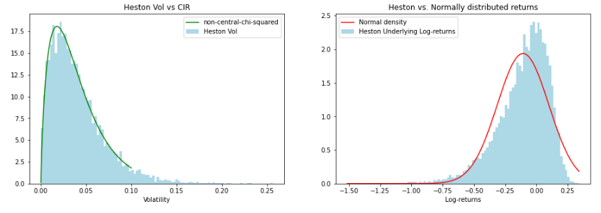
In the previous graphs, you can observe the fit (and no-fit) of the different distributions produced to known distributions assumed in other models.
Now that we have simulated all the stock prices under Heston, let’s define another function that calculates the payoffs and current price of a European call option with the following characteristics:
- $T=1$ year
- $K = 90$
- $r=0.05$
- $S_t \sim$ Heston dynamics
def heston_call_mc(S, K, r, T, t):
    payoff = np.maximum(0, S[-1, :] - K)

    average = np.mean(payoff)

    return np.exp(-r * (T - t)) * average
Note that you can improve the efficiency of the previous function substantially by implementing a better and more organized function that incorporates the generation of stock price and volatility paths. I recommend you work on this by yourself (it should be fairly easy). At this point, we just want to highlight how we apply the spirit of the Monte-Carlo method in simpler frameworks.
So, the price of a European Call option with 1 year maturity and strike 𝐾=90 (and all the other assumed parameters from before) is…
print("European Call Price under Heston: ", heston_call_mc(S, 90, 0.05, 1, 0))
European Call Price under Heston:  7.368689816806795
Comparison of Heston Option Price versus Other Methods
Let’s now see how the value of the option via Heston model differs from what we would have under the Black-Scholes framework, for example.
- Black-Scholes closed-form solution:
def bs_call_price(S, r, sigma, t, T, K):
    ttm = T - t

    if ttm < 0:
        return 0.0
    elif ttm == 0.0:
        return np.maximum(S - K, 0.0)

    vol = sigma * np.sqrt(ttm)

    d_minus = np.log(S / K) + (r - 0.5 * sigma**2) * ttm
    d_minus /= vol

    d_plus = d_minus + vol

    res = S * ss.norm.cdf(d_plus)
    res -= K * np.exp(-r * ttm) * ss.norm.cdf(d_minus)

    return res

print("European Call Price under BS: ", bs_call_price(100, 0.05, sigma_v, 0, 1, 90))
European Call Price under BS:  19.697442086839736
- Black-Scholes Monte-Carlo price:
def bs_call_mc(S, K, r, sigma, T, t, Ite):
    data = np.zeros((Ite, 2))
    z = np.random.normal(0, 1, [1, Ite])
    ST = S * np.exp((T - t) * (r - 0.5 * sigma**2) + sigma * np.sqrt(T - t) * z)
    data[:, 1] = ST - K

    average = np.sum(np.amax(data, axis=1)) / float(Ite)

    return np.exp(-r * (T - t)) * average

print(
    "European Call Price under BS (MC): ",
    bs_call_mc(100, 90, 0.05, sigma_v, 1, 0, 10000),
)
European Call Price under BS (MC):  19.71266956387397
Interestingly, we get prices that are very far away from each other. Is this a problem? Does our model not work?
Not at all! At the end of the day, why would the Heston option price converge to Black-Scholes?
-
We have already established that BS is an oversimplification of reality (remember: stylized facts!)
-
Heston (and other models) are just extending the BS world to get closer to this reality.
-
The latter seems clearer when you look at Lesson 1 and the statistical distribution under Heston. There is more kurtosis and skewness than normal distribution, just as we observe in practice.
-
If BS and Heston get to the same output, what is the point of adding mathematical and computational complexity?
There is another important issue related to model specification and parameters:
-
In the latter pricing example, we have used a $\sigma=0.3$ for both models.
-
This is not correct, since there is no easy mapping of the volatility parameter from one model to the other. In other words, the $\sigma$ parameter cannot be used interchangeably in Heston or Black-Scholes.
-
What is the real $\sigma$ for each model then? Do not worry; we will tackle this issue through calibration.
Conclusion
At the beginning of the course, we introduced a simple framework to work on, i.e., the binomial model. What we have been doing since, essentially, is advancing our understanding towards more complex models that try to capture the different features associated with underlying stock prices and returns. From Black-Scholes to the Heston model, we have merely focused on modeling the underlying price, whereas the intuition on option pricing remained intact. For the final part of the Derivative Pricing course, we will focus on one more stylized fact of stock prices: jumps.
In the next post, we will take a look at jumps in prices, as well as how can we formally model those jumps to incorporate them in our pricing.