Local Volatility Models: Dupire

Introduction

In our previous discussion, we explored the fascinating world of volatility smiles, and how they can be derived from traded option prices. Today, we’re going to take it up a notch by diving deep into the implied volatility surface—a 3D visualization that extends the concept of the volatility smile. We’ll also see how this surface is not just a function of the option’s strike price but is influenced by its maturity as well.

The Intricacies of Local Volatility Models

In mathematical finance and financial engineering, a local volatility model treats volatility as a function of both the current asset level $ S_t $ and of time $ t $. This model generalizes the Black-Scholes model, where the volatility is a constant.

Local Volatility vs. Stochastic Volatility Models

Local volatility models are often compared with stochastic volatility models. In stochastic models, the instantaneous volatility is not just a function of $ S_t $ but also depends on a new “global” randomness coming from an additional random component.

Formulation

In a local volatility model, the asset $ S_t $ that underlies a financial derivative typically follows a stochastic differential equation of the form:

\[dS_{t}=(r_{t}-d_{t})S_{t}\,dt+\sigma _{t}S_{t}\,dW_{t}\]

Here, $ r_{t} $ is the instantaneous risk-free rate, and $ W_{t} $ is a Wiener process. The amplitude of randomness is measured by the instant volatility $ \sigma_t $.

Stochastic Volatility Model

When the volatility has its own randomness—often described by a different equation driven by a different $ W $—the model is called a stochastic volatility model.

Local Volatility Model

When the volatility is merely a function of the current underlying asset level $ S_t $ and of time $ t $, we have a local volatility model. The model is then:

\[dS_{t}=(r_{t}-d_{t})S_{t}\,dt+\sigma (S_{t},t)S_{t}\,dW_{t}\]

“Local volatility” denotes the set of diffusion coefficients $ \sigma_t = \sigma(S_t, t) $ consistent with market prices for all options on a given underlying, which yields an asset price model of this type.

Application in Exotic Option Valuation

Local volatility models are used to calculate exotic option valuations which are consistent with observed prices of vanilla options.

Decoding the Implied Volatility Surface

In classical local volatility models like Dupire’s, the implied volatility is not just a function of an option’s “moneyness” (as in the Black-Scholes model) but also a function of the contract’s maturity. This makes our volatility a three-dimensional entity, graduating from a mere smile to a full-blown surface.

Setting Up the Python Environment Firstly, let’s get our Python environment up and running with the necessary modules:

from datetime import datetime
import pandas as pd
import yahoo_fin.stock_info as si
from yahoo_fin import options

For consistency, we’ll stick with IBM as our case study. Let’s fetch the future expiration dates available in the Yahoo Finance options chain:

ticker = "IBM"
options_mats = options.get_expiration_dates(ticker)
price = si.get_live_price(ticker)
print(options_mats, price)

['September 29, 2023', 'October 6, 2023', 'October 13, 2023', 'October 20, 2023', 'October 27, 2023', 'November 3, 2023', 'November 17, 2023', 'December 15, 2023', 'January 19, 2024', 'February 16, 2024', 'April 19, 2024', 'June 21, 2024', 'January 17, 2025', 'January 16, 2026']
143.1699981689453

We need to gather and format the relevant data to construct our implied volatility surface.

temp_data = pd.DataFrame()
callData = pd.DataFrame()

for time in options_mats:
    chain = options.get_options_chain(ticker, time)
    chain_df = chain["calls"]
    date_time_obj = datetime.strptime(time, "%B %d, %Y")
    Td = date_time_obj - datetime.today()

    for row in range(len(chain_df.index)):
        values_to_add = {"Matdays": Td.days, "Maturity": date_time_obj}
        values_to_add_call = {
            "Strike": chain_df["Strike"].loc[row],
            "Implied Vol": chain_df["Implied Volatility"].loc[row],
            "Price": chain_df["Last Price"].loc[row],
        }
        row_to_add = pd.Series(values_to_add)
        row_to_add_call = pd.Series(values_to_add_call)
        temp_data = temp_data.append(row_to_add, ignore_index=True)
        callData = callData.append(row_to_add_call, ignore_index=True)

callData = pd.concat([callData, temp_data], axis=1)

Plotting the Volatility Surface

import matplotlib.pyplot as plt
import numpy as np

callData["Implied Vol"] = callData["Implied Vol"].str[:-1]
callData["ImpliedVol"] = callData["Implied Vol"].astype(float)
callData = callData[callData["ImpliedVol"] < 90]
callData = callData[callData["ImpliedVol"] > 0]

fig = plt.figure(figsize=(12, 8))
ax = fig.add_subplot(111, projection="3d")
surf = ax.plot_trisurf(
    callData["Matdays"] / 365,
    np.log(callData["Strike"] / price),
    callData["ImpliedVol"] / 100,
    cmap=plt.cm.RdBu_r,
    linewidth=0,
)

ax.set_xlabel("Maturity")
ax.set_ylabel("Moneyness")
ax.set_zlabel("Implied Vol (%)")
plt.show()

Vol Surface

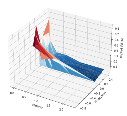
One key observation here is that the implied volatility varies for the same strike price when you consider different maturities. This multi-dimensional interplay makes the volatility surface an intriguing and essential tool for any quant.

new_df = callData[
    callData["Strike"] == 180
]  # You can change the strike if you want to see others!
new_df.head()

Strike	Implied Vol	Price	Matdays	Maturity	
107	180.0	25.00	0.01	21	    2023-10-20	
170	180.0	12.50	0.10	49	    2023-11-17	
208	180.0	6.25	0.18	112	    2024-01-19	
233	180.0	6.25	0.42	140	    2024-02-16	
252	180.0	6.25	1.00	203	    2024-04-19	

Navigating the Complexities

So, you’ve successfully constructed an implied volatility surface—congratulations! However, you might notice some anomalies like spikes in the surface, especially as you drift away from at-the-money (ATM) options. These irregularities are problematic if you are interested in pricing exotic options for which market data is not directly observable.

What Can You Do? Smoothing out the volatility surface usually involves interpolating the data, which can be quite a meticulous task. You can take a look at the following papers.

Fengler, Matthias R. “Arbitrage-Free Smoothing of the Implied Volatility Surface.” Quantitative Finance, vol. 9, no. 4, 2009, pp. 417–428.