Exploring the Volatility Smile with Yahoo Finance
Introduction
The volatility smile is a pivotal concept. Understanding it is not just an academic endeavor; it can shape trading and hedging strategies in the real world. In this post, we will demystify the construction of the volatility smile, employing data from Yahoo Finance’s option chains.
Yahoo Finance offers a treasure trove of data on exchange-traded options, both calls and puts, for an underlying stock. What is particularly interesting for us is that it provides the Black-Scholes implied volatility for varying options and strikes. This data will be instrumental throughout later, especially when calibrating models to market data.
Step 1: Delving into Volatility Data
Before diving in, let’s set up our Python environment:
from datetime import date
import yahoo_fin.stock_info as si
from yahoo_fin import options
import matplotlib.pyplot as plt
Now, let’s extract the options chain data for a specific stock. Here, we’ll use IBM as an example:
Mat = date(2023, 9, 29)
T = Mat - date.today()
ticker = "IBM"
chain = options.get_options_chain(ticker, Mat)
price = si.get_live_price(ticker)
callData = chain["calls"]
putData = chain["puts"]
callData.head(15)
In the following example, we have selected the firm IBM and will plot its volatility smile. You will have to fill in by hand the maturity date, Mat, in the code, in order to properly extract the data. You can consult the maturity you want to use here.
Then, you should fill in the Mat variable in the space given, following the form YYYY-MM-DD.
Contract Name	Last Trade Date	Strike	Last Price	Bid	Ask	Change	% Change	Volume	Open Interest	Implied Volatility
0	IBM230929C00140000	2023-08-22 9:58AM EDT	140.0	5.50	4.20	4.40	0.70	+14.58%	33	10	19.64%
1	IBM230929C00141000	2023-08-21 3:45PM EDT	141.0	4.22	3.55	3.75	0.00	-	26	25	18.99%
2	IBM230929C00142000	2023-08-17 2:31PM EDT	142.0	3.35	2.94	3.15	-0.10	-2.90%	1	2	18.38%
3	IBM230929C00143000	2023-08-15 10:11AM EDT	143.0	3.05	2.47	2.59	0.00	-	-	7	17.74%
4	IBM230929C00144000	2023-08-22 1:12PM EDT	144.0	2.25	2.03	2.14	0.10	+4.65%	1	13	17.41%
5	IBM230929C00145000	2023-08-22 2:44PM EDT	145.0	1.70	1.61	1.71	-0.25	-12.82%	13	22	16.92%
6	IBM230929C00146000	2023-08-21 3:57PM EDT	146.0	1.56	1.23	1.39	0.00	-	8	19	16.77%
7	IBM230929C00147000	2023-08-22 12:41PM EDT	147.0	1.15	0.97	1.07	0.04	+3.60%	1	53	16.32%
8	IBM230929C00148000	2023-08-22 12:17PM EDT	148.0	0.80	0.75	0.85	-0.09	-10.11%	4	18	16.25%
9	IBM230929C00149000	2023-08-17 12:50PM EDT	149.0	0.99	0.56	0.66	0.00	-	-	7	16.11%
10	IBM230929C00150000	2023-08-22 12:31PM EDT	150.0	0.54	0.44	0.51	-0.06	-10.00%	12	46	16.04%
11	IBM230929C00152500	2023-08-21 3:15PM EDT	152.5	0.30	0.23	0.27	0.00	-	1	3	16.11%
12	IBM230929C00155000	2023-08-22 2:51PM EDT	155.0	0.15	0.11	0.18	0.01	+7.14%	31	5	17.14%
13	IBM230929C00157500	2023-08-22 3:39PM EDT	157.5	0.09	0.04	0.14	0.00	-	3	3	18.56%
14	IBM230929C00165000	2023-08-17 9:47AM EDT	165.0	0.05	0.00	0.15	0.00	-	-	1	25.15%
When choosing the stock, it’s advisable to consider:
- Stocks with a high volume of exchange-traded options tend to have more robust volatility smiles.
- The ideal maturity for option contracts shouldn’t be too far in the future nor too close. A ballpark range would be around t+3 months.
- Ensure you select the exact date of the option’s expiration.
Now, let’s visualize the implied volatility smile:
df_call = callData
df_call["Implied Volatility"] = df_call["Implied Volatility"].str[:-1].astype(float)
df_call = df_call[df_call["Implied Volatility"] > 0]
df_call["Strike"] = df_call["Strike"].astype(float)
df_call = df_call[(df_call["Strike"] > price * 0.8) & (df_call["Strike"] < price * 1.2)]
df_call.plot(kind="scatter", x="Strike", y="Implied Volatility", color="red")
plt.grid()
plt.show()
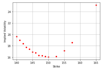
The visual might reveal not a complete smile but a smirk or skew, a phenomenon primarily arising due to increased demand for near ATM options and put options as crash hedges.
Step 2: The Newton-Raphson Method for Implied Volatility
While Yahoo Finance provides implied volatility, there’s value in understanding its derivation. The Newton-Raphson method is a popular iterative approach to this:
The Newton-Raphson method is a root-finding algorithm that seeks to find successively better approximations to the roots of a real-valued function. In the context of implied volatility, we use it to find the root of the equation:
$ C_{\text{market}} - C_{\text{BS}}(\sigma) = 0 $
Where:
- $C_{\text{market}}$ is the market price of the option.
- $C_{\text{BS}}(\sigma)$ is the Black-Scholes price of the option for a given volatility $\sigma$.
The goal is to find the implied volatility $\sigma$ that makes the Black-Scholes price as close to the market price as possible.
Steps of the Newton-Raphson Method for Implied Volatility:
-
Initialization: Start with an initial guess for implied volatility, $\sigma$. Often, this guess is something reasonable based on the market, like 20% (or 0.20).
- Compute the Price and Vega:
- Calculate the Black-Scholes price of the option using the current guess $\sigma$: $C_{\text{BS}}(\sigma)$.
- Compute the vega of the option. Vega is the sensitivity of the option’s price to changes in volatility. This is required to adjust our guess in the next step.
-
Check for Convergence: Calculate the difference between the market price and the Black-Scholes price: $\text{difference} = C_{\text{market}} - C_{\text{BS}}(\sigma)$. If this difference is smaller than a pre-defined tolerance (e.g., 0.0001), then $\sigma$ is close enough to the true implied volatility, and we stop.
-
Update the Guess: If convergence is not achieved, we update our guess for $\sigma$ using the formula: [ \sigma_{\text{new}} = \sigma_{\text{old}} - \frac{C_{\text{BS}}(\sigma_{\text{old}}) - C_{\text{market}}}{\text{vega}} ] The ratio in the formula can be thought of as the amount by which our Black-Scholes price is off, scaled by how sensitive the option price is to changes in volatility. This gives a good direction and magnitude for adjusting our guess.
-
Iterate: Return to step 2 with the new guess $\sigma_{\text{new}}$ and repeat the process.
- Stop Condition: The iteration stops either when:
- The difference between $C_{\text{market}}$ and $C_{\text{BS}}(\sigma)$ is sufficiently small (convergence is achieved).
- A maximum number of iterations is reached. This ensures the method doesn’t run indefinitely if it doesn’t converge.
First, let’s set up our mathematical tools:
import numpy as np
from scipy.stats import norm

N_prime = norm.pdf
N = norm.cdf
Now, we’ll define the Black-Scholes pricing formula for a call option:
def black_scholes_call(S, K, T, r, sigma):
    d1 = (np.log(S / K) + (r + sigma**2 / 2) * T) / (sigma * np.sqrt(T))
    d2 = d1 - sigma * np.sqrt(T)
    return S * N(d1) - N(d2) * K * np.exp(-r * T)
We also need the vega of the option:
def vega(S, K, T, r, sigma):
    d1 = (np.log(S / K) + (r + sigma**2 / 2) * T) / sigma * np.sqrt(T)
    return S * np.sqrt(T) * N_prime(d1)
Lastly, our Newton-Raphson-based function for computing implied volatility:
def implied_volatility_call(C, S, K, T, r, tol=0.0001, max_iterations=100):
    sigma = 0.3
    for i in range(max_iterations):
        diff = black_scholes_call(S, K, T, r, sigma) - C
        if abs(diff) < tol:
            return sigma
        sigma = sigma - diff / vega(S, K, T, r, sigma)
    return sigma

found on 2th iteration
difference is equal to -7.274655111189077e-06
Implied volatility using Newton Rapshon is:  0.5428424065162358
You can check the performance of this algorithm against some of the existing (freely available) online implied volatility calculators. For example, you can check this site.
Now you know a simple way to extract implied volatility from option market prices.