The Constraints of the Black-Scholes Model: A Data-Driven Analysis
The Black-Scholes model like all models, it comes with its own set of assumptions, some of which have shown to be oversimplified or even flawed. In this post, we’ll explore these assumptions and, using historical market data, analyze their shortcomings.
Assumptions of the Black-Scholes Model:
- European-style options: Can only be exercised at expiration.
- No dividends are paid out during the option’s life.
- Efficient markets: No transaction costs or taxes; all information is available to all market participants.
- Risk-free rate and volatility of the underlying are known and constant.
- Returns on the underlying are normally distributed.
- No arbitrage opportunities.
- The underlying security doesn’t pay a dividend.
- It’s possible to short-sell the underlying security without incurring a cost.
Analyzing Assumptions Using Historical Market Data
To critically evaluate some of the assumptions, we’ll fetch historical market data and analyze it against the Black-Scholes framework.
Assumption: Returns on the underlying are normally distributed.
Let’s see if this holds true for a popular stock.
import numpy as np
import pandas as pd
import yfinance as yf
import matplotlib.pyplot as plt
from scipy.stats import norm

# Setting up yfinance to fetch data
yf.pdr_override()

# Fetching data for Apple Inc. using yfinance
data = yf.download('AAPL', start='2015-01-01')

# Calculating log returns
data['Log Returns'] = np.log(data['Close'] / data['Close'].shift(1))

# Plotting the histogram of returns
plt.figure(figsize=(12,6))
plt.hist(data['Log Returns'].dropna(), bins=100, density=True, alpha=0.6, color='b')

# Plotting the normal distribution for comparison
xmin, xmax = plt.xlim()
x = np.linspace(xmin, xmax, 100)
p = norm.pdf(x, data['Log Returns'].mean(), data['Log Returns'].std())
plt.plot(x, p, 'k', linewidth=2)

title = "Fit results: mu = %.2f,  std = %.2f" % (data['Log Returns'].mean(), data['Log Returns'].std())
plt.title(title)
plt.show()
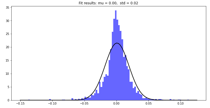
From the above plot, we can observe that real market returns often exhibit fatter tails compared to the normal distribution, challenging the assumption of normally distributed returns.
Assumption 2: Risk-free rate and volatility of the underlying are known and constant.
Let’s fetch the data using yfinance and adapt the code for plotting the rolling annual volatility and dividend payment history of Apple Inc.
Here’s the code:
import numpy as np
import pandas as pd
import yfinance as yf
import matplotlib.pyplot as plt

# Setting up yfinance to fetch data
yf.pdr_override()

# Fetching data for Apple Inc. using yfinance
data = yf.download('AAPL', start='2000-01-01')

# Calculating log returns
data['Log Returns'] = np.log(data['Close'] / data['Close'].shift(1))

# Plotting volatility (rolling standard deviation) of Apple Inc. stock returns
data['Volatility'] = data['Log Returns'].rolling(window=252).std() * np.sqrt(252)

plt.figure(figsize=(12,6))
plt.plot(data.index, data['Volatility'])
plt.title('Rolling Annual Volatility of Apple Inc.')
plt.show()
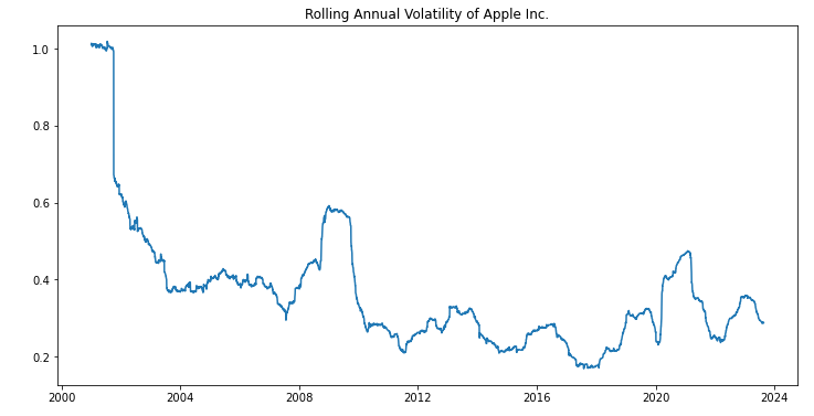
From the plot, you can see that volatility changes over time, suggesting it’s not constant.
Assumption 3: The underlying security doesn’t pay a dividend.
Fetching dividend data from Yahoo Finance using yfinance
div_data = yf.Ticker('AAPL').dividends

plt.figure(figsize=(12,6))
plt.plot(div_data.index, div_data, 'o-')  # Using 'o-' to mark dividend points
plt.title('Dividends Paid by Apple Inc.')
plt.show()
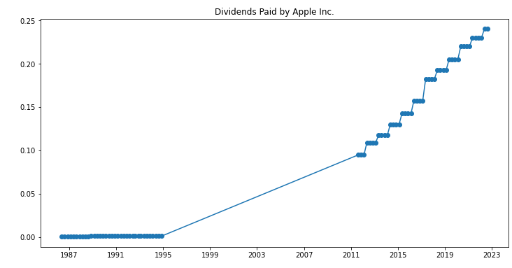
If the plot shows any peaks, it indicates dividend payments, proving that many stocks indeed pay dividends.
Conclusion
While the Black-Scholes model is a foundational pillar in financial modeling, it’s imperative to understand its limitations. As demonstrated, some of its core assumptions don’t always align with real market behavior.
You can then extend this analysis for the rest of the assumptions. Some of them might not be easily disproven with data alone and might require a more theoretical or qualitative analysis.