Simulating Interest Rates: Vasicek Model
We will tackle the use of stochastic differential equations (SDE) for simulating the behavior of other types of assets. Specifically, we will focus on simulating interest rates using the SDE associated with the Vasicek (1977) model.
As always, let’s first import some libraries we will need down the road:
import matplotlib.pyplot as plt
import numpy as np
import pandas_datareader as pdr
1. Vasicek (1977) Model
The Vasicek interest rate model can be described as: \begin{equation} dr = k(\theta - r) \, dt + \sigma \, dz \end{equation}
- r is the short interest rate.
- k is the speed of reversion to the mean. It dictates how rapidly the interest rate r.
- r reverts to its long-term mean value θ.
- θ is the long-term mean level of the interest rate. The rate r.
- r will tend to revert to this value over time.
- σ is the volatility of the interest rate, defining the standard deviation of changes in the interest rate.
- dz is the change in a Wiener process or standard Brownian motion.
These parameters would typically be estimated or calibrated using market data when applying the model.
Let’s build a function for this SDE:
# Vasicek (1977) Model
# Vasicek's risk-neutral process for interest rates is given by:
# dr = k(θ-r)dt + σdz, where dz = √dt * z, with z ~ N(0,1)

def vasicek(r0, K, theta, sigma, T, N, M):
    dt = T / N
    rates = np.zeros((N, M))
    rates[0, :] = r0
    for j in range(M):
        for i in range(1, N):
            dr = (
                K * (theta - rates[i - 1, j]) * dt
                + sigma * np.sqrt(dt) * np.random.normal()
            )
            rates[i, j] = rates[i - 1, j] + dr
    return rates
We are fetching historical 3-month Treasury bill rates as a representative of short-term interest rates. The most recent value from this data is then used as in the Vasicek model simulation. Adjust the start parameter in the DataReader function if you wish to fetch data from a different starting date.
# Downloading historical 3-month Treasury bill rates from FRED as a representation of short-term interest rates
data = pdr.data.DataReader('TB3MS', 'fred', start='2000-01-01')  # TB3MS is the FRED code for 3-month T-bill secondary market rate
latest_rate = data.iloc[-1, 0] / 100  # Convert the rate from percentage to decimal
r0 = latest_rate
Now, we can use the same intuition of the Monte Carlo methods we used before for the Black-Scholes SDE to simulate interest rates given a current level, $r_0$.
M = 100  # Number of paths for MC
N = 100  # Number of steps
T = 2.0  # Maturity
K = 0.40
theta = 0.01
sigma = 0.012
t = np.linspace(0, T, N)

rates = vasicek(r0, K, theta, sigma, T, N, M)
rates.shape
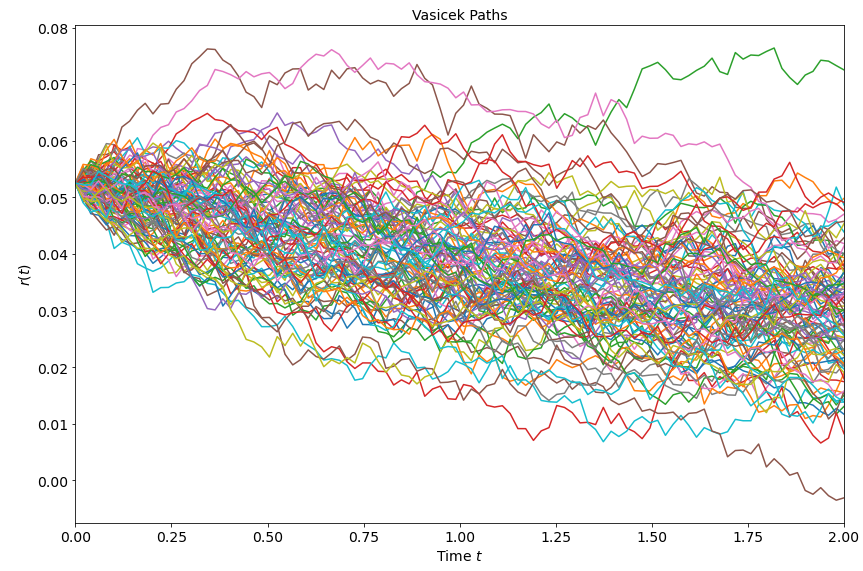
We have simulated interest rates for 100 paths and 100 steps.
Let’s see how these look:
plt.figure(figsize=(12, 8))
for j in range(M):
    plt.plot(t, rates[:, j])

plt.xlabel("Time $t$", fontsize=14)
plt.ylabel("$r(t)$", fontsize=14)
plt.title("Vasicek Paths", fontsize=14)
axes = plt.gca()
axes.set_xlim([0, T])
plt.xticks(fontsize=14)
plt.yticks(fontsize=14)
plt.tight_layout()
plt.show()
Conclusion
The Vasicek model and other interest rate models are vital tools in finance for several reasons:
-
Fixed-Income Pricing: The most direct application is in the pricing of fixed-income securities, especially those with embedded options like callable or puttable bonds. The future cash flows of such instruments depend on the path of interest rates, making it essential to have a reliable model to simulate these paths.
-
Risk Management: Financial institutions, particularly banks, are highly sensitive to interest rate movements. They need to quantify how shifts in rates might impact their portfolios. Interest rate models can help in measuring interest rate risk, such as value at risk (VaR) or potential future exposure.
-
Derivatives Pricing: Interest rate derivatives like caps, floors, swaptions, and structured products rely heavily on the evolution of interest rates. Accurate simulation and modeling of the term structure are crucial for pricing and risk-managing these instruments.
-
*Hedging Strategies: Interest rate models can guide traders and treasurers in devising hedging strategies to protect against adverse movements in rates.
-
Economic Forecasting: Central banks and economic researchers might use (more complex) interest rate models as a part of larger macroeconomic models to forecast economic variables and guide policy decisions.
It’s important to note, however, they have been built upon and extended in numerous ways to better capture the complexities of real-world interest rate movements. Models like the Cox-Ingersoll-Ross (CIR), Hull-White, and the LIBOR Market Model are examples of these advancements.