Markov's Property and Geometric Brownian Motion
Intoruction
In this module, we extend the option-pricing concepts from our earlier discussions into a continuous-time framework. Our initial step involves understanding the kind of stochastic process that will serve as our model for stock prices. Similar to how we constructed various paths in the binomial framework, we are now set to build “paths” that emulate the future behavior of stock prices.
Generating Consistent Random Numbers
To kick things off, let’s examine how we can define random numbers that follow a Wiener process (or Brownian motion) using Python. The numpy module’s random.randn function allows us to generate random numbers from a standard normal distribution ~N(0,1).
import numpy as np

X = np.random.randn(100)
print(X)
Every time we run this code, the output changes due to the randomness. However, sometimes, especially when comparing different results and modeling approaches, it’s valuable to work with a consistent set of “random” numbers.
Random numbers in Python are produced algorithmically and are not genuinely random. These algorithms utilize a “random” seed as input and produce random numbers from it. Consequently, if we set the initial seed to a constant value, the output of np.random.rand(n) will consistently be the same.
np.random.seed(10)
X = np.random.randn(100)
print(X)
Run the above code multiple times and observe that the random numbers generated remain the same, as long as we don’t alter the seed.
Simulating Stock Price Paths: The Geometric Brownian Motion (GBM)
Next, let’s utilize these random numbers to simulate stock price paths under a GBM process. The equations for GBM, given below, are what we use to model stock price movements in continuous time:
\[dS = S_0 \left(\mu dt + \sigma dW_t \right)\]Here is how we can simulate these paths in Python:
import matplotlib.pyplot as plt

fig = plt.figure()

T = 1  # years
N = 255  # Number of points, number of subintervals = N-1
dt = T / N  # Time step in "years"
t = np.linspace(0, T, N)
M = 100  # Number of paths (Monte Carlo approach)
vol = 0.18
S0 = 10
mu = 0.08  # drift

dS = S0 * (mu * dt + vol * np.sqrt(dt) * np.random.randn(M, N))
S = S0 + np.cumsum(dS, axis=1)

for i in range(M):
    plt.plot(t, S[i, :])

plt.xlabel("Time $t$", fontsize=14)
plt.ylabel("Random Variable $S(t)$", fontsize=14)
plt.title("GBM Paths", fontsize=14)
axes = plt.gca()
axes.set_xlim([0, T])
plt.xticks(fontsize=14)
plt.yticks(fontsize=14)
plt.tight_layout()
plt.show()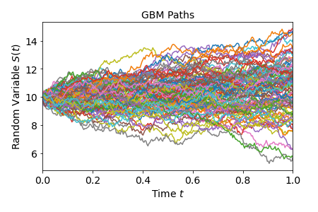
In the plots above, the various paths generated with the GBM stochastic differential equation (SDE) are represented.
Now, let’s inspect how the returns from these simulated price paths appear in a histogram:
Returns = (S[:, -1] - S[:, 0]) / S[:, 0]
plt.hist(Returns, bins=25)
plt.axvline(np.percentile(Returns, 10), color="r", linestyle="dashed", linewidth=2)
plt.axvline(np.percentile(Returns, 90), color="r", linestyle="dashed", linewidth=2)
plt.show()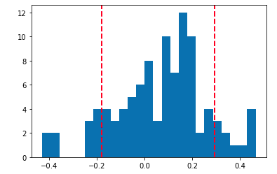
This gives us a complete distribution of the simulated returns, revealing some of its characteristics. One simple analysis involves using risk metrics like Value at Risk (VaR), which measures the maximum drop in returns at a given confidence level:
print(np.percentile(Returns, 5)) # Value at Risk at 5%In this scenario, given the parameters of the GBM equation and simulated prices and returns, we might infer that with 95% probability, the stock will not drop more than 22% in a given day.
Conclusion
We ventured into generating random numbers and used them to simulate stock price paths employing the Geometric Brownian Motion (GBM) equation. We then visualized these paths and analyzed the distribution of simulated returns, giving us insights that can be quantified using risk metrics like VaR.
As we progress, we will delve deeper into more sophisticated models that account for real-world market behavior, such as sudden price jumps. In the upcoming post, we will explore how to analytically solve the SDE for the GBM process using Itô calculus.
Note
Remember the analytical solution of the GBM SDE isn’t just a mathematical novelty; it’s a cornerstone of modern financial theory and practice.
The Black-Scholes formula, the bedrock of modern option pricing, is derived from the analytical solution of the GBM. Without a closed-form solution for the GBM, the Black-Scholes model wouldn’t exist in its current form.
Whether you’re pricing complex derivatives, managing a portfolio’s risk, or trying to predict future stock prices, the analytical solution provides clarity, speed, and a deeper understanding of the underlying financial dynamics.