Calibration of the Binomial Option Pricing Model
In this post, we will focus on calibrating the Binomial Option Pricing Model (BOPM) using the underlying asset’s volatility. This is a vital step in derivative pricing and can have substantial implications for trading and risk management.
Adjusting u and d for Underlying Volatility
The up u and down d factors in the BOPM are adjusted to match the underlying stock’s volatility. These adjustments are given by:
Where:
-
σis the volatility of the stock -
dtis the time increment which equalsT/N, whereTis the time to expiration andNis the number of time steps in the binomial tree.
For instance, consider we have a known underlying stock volatility of 30% for the next year.
Below is the Python function call_option_delta which calculates the call option price and Delta, incorporating the volatility adjustments to u and d:
import numpy as np

def call_option_delta(S_ini, K, T, r, sigma, N):
    dt = T / N  # Define time step
    u = np.exp(sigma * np.sqrt(dt))  # Define u
    d = np.exp(-sigma * np.sqrt(dt))  # Define d
    p = (np.exp(r * dt) - d) / (u - d)  # risk neutral probs
    C = np.zeros([N + 1, N + 1])  # call prices
    S = np.zeros([N + 1, N + 1])  # underlying price
    Delta = np.zeros([N, N])  # delta
    for i in range(0, N + 1):
        C[N, i] = max(S_ini * (u ** (i)) * (d ** (N - i)) - K, 0)
        S[N, i] = S_ini * (u ** (i)) * (d ** (N - i))
    for j in range(N - 1, -1, -1):
        for i in range(0, j + 1):
            C[j, i] = np.exp(-r * dt) * (p * C[j + 1, i + 1] + (1 - p) * C[j + 1, i])
            S[j, i] = S_ini * (u ** (i)) * (d ** (j - i))
            Delta[j, i] = (C[j + 1, i + 1] - C[j + 1, i]) / (
                S[j + 1, i + 1] - S[j + 1, i]
            )
    return C[0, 0], C, S, Delta

call_price, C, S, delta =call_option_delta(100, 90, 1, 0, 0.3, 10)
Let’s see the graphical representation of our tree.
import matplotlib.pyplot as plt

def plot_binomial_tree(S, C):
    N = S.shape[0]
    fig, ax = plt.subplots(2, 1, figsize=(10, 12))

    # Function to plot tree
    def plot_tree(ax, data, title, color):
        for i in range(N):
            for j in range(i + 1):
                x = j - i/2  # Adjust x coordinates for tree shape
                y = N - i   # Adjust y coordinates to start from the bottom
                ax.plot(x, y, 'o', color=color)
                ax.text(x, y, f'{data[i,j]:.2f}', ha='center', va='center', fontsize=10, bbox=dict(facecolor='white', edgecolor='white', boxstyle='circle'))
                if i < N - 1:  # Draw connecting lines only for non-terminal nodes
                    ax.plot([x, x - 0.5], [y, y - 1], 'k-')  # Line for downward movement
                    ax.plot([x, x + 0.5], [y, y - 1], 'k-')  # Line for upward movement
        ax.set_title(title)
        ax.axis('off')

    # Plot underlying and option prices
    plot_tree(ax[0], S, "Underlying Prices", 'blue')
    plot_tree(ax[1], C, "Option Prices", 'red')

    plt.tight_layout()
    plt.show()

# Call the plotting function
plot_binomial_tree(S, C)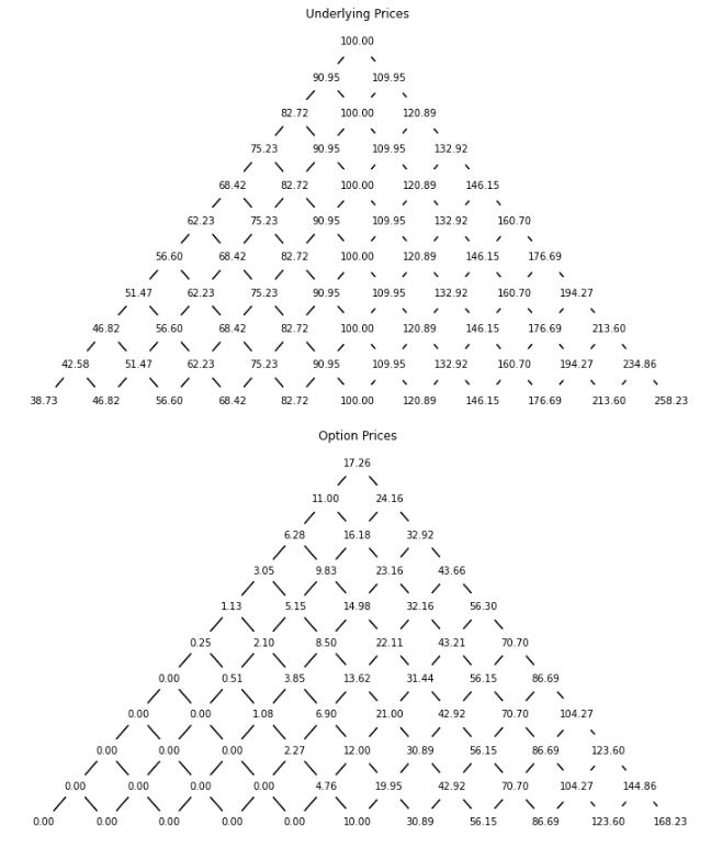
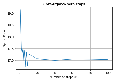
Convergence Analysis
We analyze the effect of varying N, the number of time steps, on the computed option price.
As N increases, the computed option price should converge to a stable value.
For example, with parameters K=90, r=0%, T=1, σ=0.3, we observed a clear convergence of the option price to $17.01 as N increases.
Here is the Python code for the convergence analysis:
price_array = []
N_values = [1, 2, 3, 4, 5, ..., 1000]
for N in N_values:
    call_price, _, _, _ = call_option_delta(100, 90, 1, 0, 0.3, N)
    price_array.append(call_price)
    print("With N = {:3d}, the price is {:.2f}".format(N, call_price))
With N = 1, the price is 19.14
With N = 2, the price is 17.51
With N = 3, the price is 17.28
With N = 4, the price is 17.50
With N = 5, the price is 16.90
With N = 6, the price is 17.41
With N = 7, the price is 16.73
With N = 8, the price is 17.33
With N = 9, the price is 16.76
With N = 10, the price is 17.26
With N = 20, the price is 17.06
With N = 40, the price is 16.99
With N = 60, the price is 17.05
With N = 80, the price is 17.04
With N = 100, the price is 17.02
With N = 200, the price is 17.03
With N = 300, the price is 17.01
With N = 400, the price is 17.02
With N = 500, the price is 17.01
With N = 600, the price is 17.02
With N = 700, the price is 17.02
With N = 800, the price is 17.01
With N = 900, the price is 17.01
With N = 1000, the price is 17.02And the graphical representation:
import matplotlib.pyplot as plt

plt.plot(N_values, price_array)
plt.title("Convergence with steps")
plt.xlabel("Number of steps (N)")
plt.ylabel("Option Price")
plt.grid(True)
plt.show()
Obtaining Volatility σ
A critical and challenging step is to obtain σ, the volatility of the underlying asset. This can be sourced in a couple of ways:
-
Historical Asset Volatility: This involves computing the volatility based on past stock price movements. However, it assumes that past behavior predicts future behavior, which is not always accurate.
-
Implied Asset Volatility: This is inferred from the prices of traded options. Essentially, given an option’s market price and using a pricing model, we solve for the volatility that reconciles the model price with the market price. This is often the most reliable estimate of the market’s expectation of future volatility.
Conclusion
In this post, we discussed the essential concept of calibrating the BOPM using the underlying asset’s volatility, illustrated with a Python implementation. Model calibration is a crucial step in options pricing as it aligns the model’s assumptions with observable market data. As we progress into more complex derivatives and models, calibration will remain a foundational concept.
In the upcoming posts, we will extend these ideas to American options, which introduces additional complexities and opportunities for calibration.