Binomial Model
Understanding the Binomial Tree Model for Pricing Options
When it comes to pricing options, understanding the binomial tree model is crucial. In this article, we’ll discuss how this model operates and demonstrate how to implement it using Python.
The binomial model is a discrete model used in calculating the value of options. The core concept is constructing a binomial tree, which is a graphical representation of possible intrinsic values an option may take at different times.
Steps to calculate the option price using backward induction:
Terminal Payoffs: At the final nodes of the binomial tree (at expiration), the option value is straightforward to determine. It is simply the intrinsic value of the option.
For a European Call: max(S−K,0) For a European Put: max(K−S,0)
Where S S is the stock price and K K is the strike price.
Backward Induction: Once we have the terminal option values, we move one step backward in the tree and calculate the option value at each preceding node. We use the concept of risk-neutral valuation to do this.
Iterate Backward: We repeat the above step, working backward from the option’s expiration to the present, node by node, until we reach the very first node, which gives us the option’s current market value.
Before we start, we’ll need to import the numpy library as it provides tools for working with arrays which are essential for our calculations.
import numpy as npWe need several inputs to compute the binomial tree: upward movement (u), downward movement (d), risk-free rate (rf), time-horizon (T), and number of steps in the tree (N). All these are user-inputs for our function.
One important point is the concept of time-step. The time-step (dt) in our binomial model represents how long does moving from one node to the next one in the tree represent in terms of time? It’s calculated as T/N.
Constructing a Binomial Tree
Here’s a Python function that simulates the underlying stock price given some inputs: initial stock price (S_ini), time-horizon (T), upward (u) and downward (d) movements, and number of steps (N).
def binomial_tree(S_ini, T, u, d, N):
    S = np.zeros([N + 1, N + 1])  # Underlying price
    for i in range(0, N + 1):
        S[N, i] = S_ini * (u ** (i)) * (d ** (N - i))
    for j in range(N - 1, -1, -1):
        for i in range(0, j + 1):
            S[j, i] = S_ini * (u ** (i)) * (d ** (j - i))
    return S
Extending the Tree with Call Option Payoffs
We can extend the function by adding another variable that computes the payoffs associated with a Call Option. Here, we’re focusing on a European Call Option with a specific strike price (K).
def binomial_tree_call(S_ini, K, T, u, d, N):
    C = np.zeros([N + 1, N + 1])  # Call prices
    S = np.zeros([N + 1, N + 1])  # Underlying price
    for i in range(0, N + 1):
        C[N, i] = max(S_ini * (u ** (i)) * (d ** (N - i)) - K, 0)
        S[N, i] = S_ini * (u ** (i)) * (d ** (N - i))
    for j in range(N - 1, -1, -1):
        for i in range(0, j + 1):
            S[j, i] = S_ini * (u ** (i)) * (d ** (j - i))
    return S, C
Introducing Risk-Neutral Probabilities and Backward Induction
Lastly, let’s work with risk-neutral probabilities. Once we have the probabilities, we can use backward induction to calculate the value of the Call Option at each node.
def binomial_call_full(S_ini, K, T, r, u, d, N):
    dt = T / N  # Define time step
    p = (np.exp(r * dt) - d) / (u - d)  # Risk neutral probabilities (probs)
    C = np.zeros([N + 1, N + 1])  # Call prices
    S = np.zeros([N + 1, N + 1])  # Underlying price
    for i in range(0, N + 1):
        C[N, i] = max(S_ini * (u ** (i)) * (d ** (N - i)) - K, 0)
        S[N, i] = S_ini * (u ** (i)) * (d ** (N - i))
    for j in range(N - 1, -1, -1):
        for i in range(0, j + 1):
            C[j, i] = np.exp(-r * dt) * (p * C[j + 1, i + 1] + (1 - p) * C[j + 1, i])
            S[j, i] = S_ini * (u ** (i)) * (d ** (j - i))
    return C[0, 0], C, S
Let’s suppose you have the following parameters for a binomial option:
- Initial Stock price (
S_ini): $100 - Strike price (
K): $100 - Time to maturity in years (
T): 1 - Risk-free interest rate (
r): 5% (0.05) - Upward price movement (
u): 1.2 - Downward price movement (
d): 0.8 - Number of periods (
N): 3
C0, C, S = binomial_call_full(100, 100, 1, 0.05, 1.2, 0.8, 3)
C0: This is the price of the option at the initial time (t=0).
C: This is a 2D numpy array that contains the price of the option at each node of the binomial tree. Each row in this array corresponds to a time step, and each column corresponds to a state (number of upward movements).
S: This is a 2D numpy array that contains the price of the underlying stock at each node of the binomial tree. Each row in this array corresponds to a time step, and each column corresponds to a state (number of upward movements).
C0 = 16.863001872208116print("Option Prices at each node: ")
for i in range(len(C)):
print(' ' * (len(C) - i - 1), end='')
for j in range(i+1):
print("{:.2f} ".format(C[i, j]), end='')
print()
print("\nUnderlying Prices at each node: ")
for i in range(len(S)):
print(' ' * (len(S) - i - 1), end='')
for j in range(i+1):
print("{:.2f} ".format(S[i, j]), end='')
print()Option Prices at each node:
16.86
4.32 27.99
0.00 8.10 45.65
0.00 0.00 15.20 72.80 Underlying Prices at each node:
100.00
80.00 120.00
64.00 96.00 144.00
51.20 76.80 115.20 172.80 This function incorporates all the factors we discussed and gives the Call Option price today. We achieve this by doing backward induction from the last period (maturity) and work backwards.
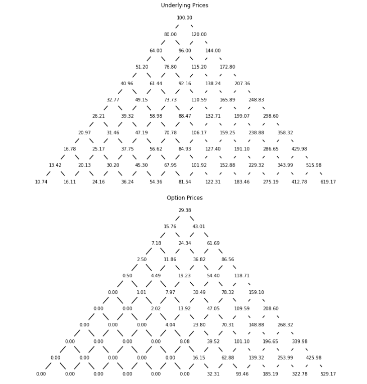
Binomial Model Convergence
A key strength of the Binomial Option Pricing Model is its mathematical robustness and flexibility. In fact, as the number of steps in the binomial tree increases to infinity, the Binomial Option Pricing Model converges to the Black-Scholes-Merton Model, one of the cornerstones in the field of financial derivatives pricing.
We have the time step calculation:
\[dt = \frac{T}{N}\]The risk-neutral probability calculation:
\[p = \frac{e^{r \cdot dt} - d}{u - d}\]For each node $(i, j)$ in the tree, where $i$ represents the time step and $j$ represents the state (number of upward movements), we calculate the call option price $C[i, j]$ and the stock price $S[i, j]$:
At the final time step $(i=N)$, we have:
\[C[N, j] = \max[S_{\text{ini}} \cdot u^{j} \cdot d^{N - j} - K, 0]\] \[S[N, j] = S_{\text{ini}} \cdot u^{j} \cdot d^{N - j}\]At all earlier time steps $(i < N)$, we have:
\[C[i, j] = e^{-r \cdot dt} \cdot [p \cdot C[i + 1, j + 1] + (1 - p) \cdot C[i + 1, j]]\] \[S[i, j] = S_{\text{ini}} \cdot u^{j} \cdot d^{i - j}\]Note that the indices $i$ and $j$ are integer values, with $i$ going from $0$ to $N$ and $j$ going from $0$ to $i$ at each step. The $\max$ function in the equation for $C[N, j]$ represents the intrinsic value of the call option, which is the maximum of the stock price minus the strike price and zero.
Finally, the function returns $C[0, 0]$, $C$, and $S$, where $C[0, 0]$ represents the option price at $t=0$, and $C$ and $S$ represent the option prices and stock prices at each node in the binomial tree, respectively.