Merton model
Introduction
The Merton model is an extension of the Black-Scholes model, incorporating both stochastic volatility and jumps in asset prices. It provides a more realistic representation of asset price dynamics by capturing sudden, significant changes in asset values that occur in real markets. Here are the key concepts and assumptions:
Key Concepts:
-
Jump-Diffusion Process: The Merton model assumes that asset prices follow a jump-diffusion process, which is essentially a combination of a geometric Brownian motion and a Poisson jump process.
-
Stochastic Differential Equation (SDE): The model is usually defined as a stochastic differential equation that includes terms for both continuous price movements and jumps.
-
Risk-Neutral Pricing: Like the Black-Scholes model, the Merton model operates under a risk-neutral measure, meaning that all assets are assumed to grow at the risk-free rate when pricing derivatives.
-
Volatility: The model accounts for the asset’s volatility, but unlike models like Heston or Bates, it assumes that the volatility remains constant over time.
-
Jump Intensity: The model introduces a new parameter, ( \lambda ), which represents the frequency of jumps expected to occur in a given period.
-
Jump Size: Jump sizes are assumed to follow a log-normal distribution, characterized by parameters ( \mu_j ) (mean) and ( \delta ) (volatility).
The Merton model offers a more nuanced picture of asset price behavior compared to the Black-Scholes model. However, it also introduces additional complexity, particularly when calibrating the model to market data due to the additional parameters associated with the jump component.
We will implement the Merton (1976) jump diffusion model in Python using Monte Carlo methods. Then, we will discuss the comparison with the Black-Scholes framework and the meaning and interpretation of the different parameters.
As usual, let’s start by importing the necessary libraries:
import matplotlib.pyplot as plt
import numpy as np
import scipy.stats as ss
1. Implementing the Merton Model
We will start by implementing the Merton model in Python. As you already know, the model has the following SDE: \(\begin{equation*} dS_t = \left( r - r_j \right) S_t dt + \sigma S_t dZ_t + J_t S_t dN_t \end{equation*}\) with the following discretized form: \(\begin{equation*} S_t = S_{t-1} \left( e^{\left(r-r_j-\frac{\sigma^2}{2}\right)dt + \sigma \sqrt{dt} z_t^1}+ \left(e^{\mu_j+\delta z_t^2}-1 \right) y_t \right) \end{equation*}\) where $z_t^1$ and $z_t^2$ follow a standard normal and $y_t$ follows a Poisson process. Finally, $r_j$ equals to: \(\begin{equation*} r_j = \lambda \left(e^{\mu_j+\frac{\delta^2}{2}}\right)-1 \end{equation*}\) The Merton model is a jump-diffusion model that generalizes the Black-Scholes model by incorporating stochastic volatility and jumps in asset prices. Below are the key parameters and concepts:
Parameters:
-
$ S_t $: The stock price at time $ t $.
-
$ r $: The risk-free interest rate.
-
$ r_j $: A correction term for the jump process, defined by $ \lambda \left(e^{\mu_j+\frac{\delta^2}{2}}\right)-1 $.
-
$ \sigma $: Volatility of the underlying asset price.
-
$ \mu_j $: Mean of the log-normal distribution governing the size of the jump.
-
$ \delta $: Volatility of the log-normal distribution governing the size of the jump.
-
$ \lambda $: The intensity or frequency of jumps, essentially representing how often jumps are expected to occur in a given time period.
-
$ dZ_t $: The standard Brownian motion or Wiener process.
-
$ dN_t $: The Poisson process indicating the arrival of jumps.
Wrapping up
-
Stochastic Differential Equation (SDE): The equation describes the evolution of the stock price incorporating both a diffusion term (stochastic volatility) and a jump term.
-
Discretized Form: The SDE is discretized for numerical simulations like Monte Carlo.
-
Calibration: Parameters are typically calibrated to existing market data, often by minimizing the difference between model-generated prices and observed market prices for a set of options.
-
Brownian Motion $ dZ_t $: Represents the continuous movement of the stock price.
-
Poisson Process $ dN_t $: Describes the occurrence of jumps at any given time.
-
Jump Correction $ r_j $: A term designed to correct the expected return for the impact of jumps.
Remember that, in order to obtain the parameters of the model, we will perform an exercise of calibration to option market prices. For now, let’s assume these parameters as given and equal to:
lamb = 0.75  # Lambda of the model
mu = -0.6  # Mu
delta = 0.25  # Delta
Let’s also assume the following information for the current stock price, number of simulations in our Monte Carlo estimations, etc.
r = 0.05 # Risk-free rate
sigma = 0.2 # Volatility
T = 1.0 # Maturity/time period (in years)
S0 = 100 # Current Stock Price
Ite = 10000 # Number of simulations (paths)
M = 50 # Number of steps
dt = T / M # Time-step
Next, we will calculate the random numbers that we need, together with some variable definitions for later on:
SM = np.zeros((M + 1, Ite))
SM[0] = S0
# rj
rj = lamb * (np.exp(mu + 0.5 * delta**2) - 1)
# Random numbers
z1 = np.random.standard_normal((M + 1, Ite))
z2 = np.random.standard_normal((M + 1, Ite))
y = np.random.poisson(lamb * dt, (M + 1, Ite))
With this info, and using the Monte Carlo methods we are familiar with already, we can simulate paths for our stock price under Merton SDE:
for t in range(1, M + 1):
    SM[t] = SM[t - 1] * (
        np.exp((r - rj - 0.5 * sigma**2) * dt + sigma * np.sqrt(dt) * z1[t])
        + (np.exp(mu + delta * z2[t]) - 1) * y[t]
    )
    SM[t] = np.maximum(
        SM[t], 0.00001
    )  # To ensure that the price never goes below zero!
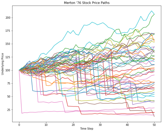
Let’s see how stock price evaluation looks for a sample of 50 paths.
plt.figure(figsize=(10, 8))
plt.plot(SM[:, 100:150])
plt.title("Merton '76 Stock Price Paths")
plt.xlabel("Time Step")
plt.ylabel("Underlying Price")
plt.show()
What is the distribution of stock returns that this model produces?
retSM = np.log(SM[-1, :] / S0)
x = np.linspace(retSM.min(), retSM.max(), 500)

plt.figure(figsize=(12, 8))
plt.hist(retSM, density=True, bins=500)
plt.plot(
    x, ss.norm.pdf(x, retSM.mean(), retSM.std()), color="r", label="Normal density"
)
plt.legend()
plt.show()
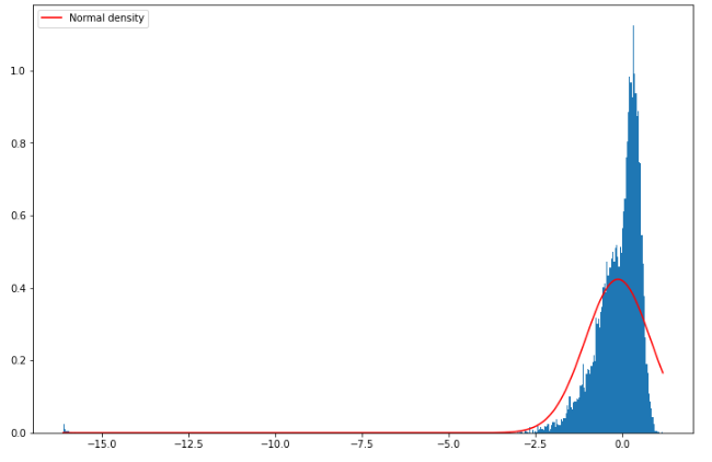
As you can see, the distribution generated by the Merton model has more kurtosis than a normal distribution and a negative skewness, consistent with the different stylized facts of stock returns. We will, later on, discuss how changing the different parameters modifies this distribution.
Comparison to Heston and GBM Returns
Next, we will compare the return (and its distribution) generated by other models like Black-Scholes (GBM) or Heston.
Let’s start with the former and, when possible, use the same parameters as in the previous example.
GBM Returns and Distribution
Let’s implement the classic GBM and check the distribution of its returns:
S = np.zeros((M + 1, Ite))
S[0] = S0
for t in range(1, M + 1):
    S[t] = S[t - 1] * np.exp(
        (r - 0.5 * sigma**2) * dt
        + sigma * np.sqrt(dt) * np.random.standard_normal(Ite)
    )

retS = np.log(S[-1, :] / S0)
y = np.linspace(retS.min(), retS.max(), 500)

plt.figure(figsize=(12, 8))
plt.hist(retS, density=True, bins=500)
plt.plot(y, ss.norm.pdf(y, retS.mean(), retS.std()), color="r", label="Normal density")
plt.legend()
plt.show()
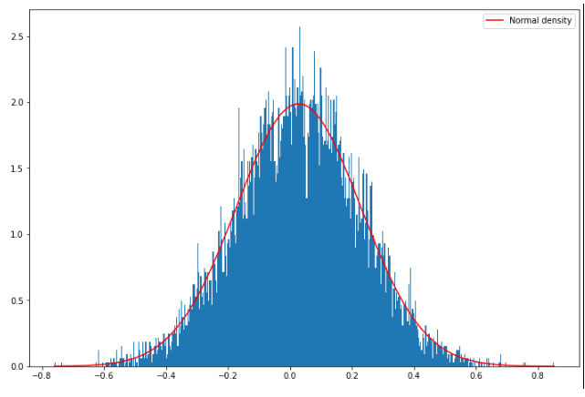
Obviously, what we get here is the classic normal distribution.
Heston Returns and Their Distribution
Finally, let’s compare this to Heston-produced returns:
def SDE_vol(v0, kappa, theta, sigma, T, M, Ite, rand, row, cho_matrix):
    dt = T / M  # T = maturity, M = number of time steps
    v = np.zeros((M + 1, Ite), dtype=np.float)
    v[0] = v0
    sdt = np.sqrt(dt)  # Sqrt of dt
    for t in range(1, M + 1):
        ran = np.dot(cho_matrix, rand[:, t])
        v[t] = np.maximum(
            0,
            v[t - 1]
            + kappa * (theta - v[t - 1]) * dt
            + np.sqrt(v[t - 1]) * sigma * ran[row] * sdt,
        )
    return v
def Heston_paths(S0, r, v, row, cho_matrix):
S = np.zeros((M + 1, Ite), dtype=float)
S[0] = S0
sdt = np.sqrt(dt)
for t in range(1, M + 1, 1):
ran = np.dot(cho_matrix, rand[:, t])
S[t] = S[t - 1] * np.exp((r - 0.5 * v[t]) * dt + np.sqrt(v[t]) * ran[row] * sdt)
return S
def random_number_gen(M, Ite):
rand = np.random.standard_normal((2, M + 1, Ite))
return rand
# Heston given parameters
v0 = 0.04
kappa_v = 2
sigma_v = 0.2
theta_v = 0.04
rho = -0.9
# Generating random numbers from standard normal
rand = random_number_gen(M, Ite)
# Covariance Matrix
covariance_matrix = np.zeros((2, 2))
covariance_matrix[0] = [1.0, rho]
covariance_matrix[1] = [rho, 1.0]
cho_matrix = np.linalg.cholesky(covariance_matrix)
# Volatility process paths
V = SDE_vol(v0, kappa_v, theta_v, sigma_v, T, M, Ite, rand, 1, cho_matrix)
# Underlying price process paths
HS = Heston_paths(S0, r, V, 0, cho_matrix)
retHS = np.log(HS[-1, :] / S0)
q = np.linspace(retHS.min(), retHS.max(), 500)
plt.figure(figsize=(12, 8))
plt.hist(retHS, density=True, bins=500)
plt.plot(
q, ss.norm.pdf(y, retHS.mean(), retHS.std()), color="r", label="Normal density"
)
plt.legend()
plt.show()
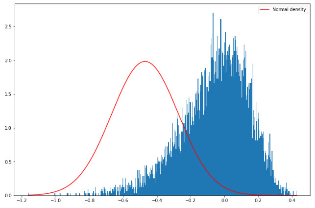
As we have seen in the previous posts, this is the distribution of returns produced by Heston.
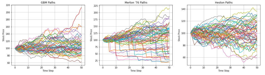
These clear differences between the different models are also evident just by looking at the kind of stock price paths they produce:
fig = plt.figure(figsize=(20, 5))
ax1 = fig.add_subplot(131)
ax2 = fig.add_subplot(132)
ax3 = fig.add_subplot(133)
ax1.plot(S[:, :50])
ax1.grid()
ax1.set_title("GBM Paths")
ax1.set_ylabel("Stock Price")
ax1.set_xlabel("Time Step")
ax2.plot(SM[:, :50])
ax2.grid()
ax2.set_title("Merton '76 Paths")
ax2.set_ylabel("Stock Price")
ax2.set_xlabel("Time Step")
ax3.plot(HS[:, :50])
ax3.grid()
ax3.set_title("Heston Paths")
ax3.set_ylabel("Stock Price")
ax3.set_xlabel("Time Step")
Text(0.5, 0, 'Time Step')
Option Pricing under the Different Models
Next, let’s explore the consequences of these differences in option pricing. For simplicity, let’s assume a European call option with 𝐾=90 and 𝑇=1 year. Let’s use Monte Carlo methods for this and assume the parameters from before.
Pricing under Black-Scholes (GBM)
def bs_call_mc(S, K, r, sigma, T, t, Ite):
data = np.zeros((Ite, 2))
z = np.random.normal(0, 1, [1, Ite])
ST = S * np.exp((T - t) * (r - 0.5 * sigma**2) + sigma * np.sqrt(T - t) * z)
data[:, 1] = ST - K
average = np.sum(np.amax(data, axis=1)) / float(Ite)
return np.exp(-r * (T - t)) * average
print("European Call Price under BS (MC): ", bs_call_mc(S0, 90, r, sigma, T, 0, Ite))
European Call Price under BS (MC): 16.537389437608663
Pricing under Heston
def heston_call_mc(S, K, r, T, t):
payoff = np.maximum(0, S[-1, :] - K)
average = np.mean(payoff)
return np.exp(-r * (T - t)) * average
print("European Call Price under Heston: ", heston_call_mc(HS, 90, r, T, 0))
European Call Price under Heston: 10.405963761175071
Pricing under Merton
def merton_call_mc(S, K, r, T, t):
payoff = np.maximum(0, S[-1, :] - K)
average = np.mean(payoff)
return np.exp(-r * (T - t)) * average
print("European Call Price under Merton: ", merton_call_mc(SM, 90, r, T, 0))
European Call Price under Merton: 27.44907468043429
Are these results for the price of the options consistent with the distributions we observed?
Discussion of Merton Model Parameters
Finally, let’s discuss empirically how the different parameters from Merton influence the type and form of the distribution of stock returns. Specifically, we will focus on the parameters $\lambda$ and $\mu_j$:
-
$\lambda$ → Intensity (frequency) of the jump (shock) to stock prices
-
$\mu_j$ → Average jump size (can be positive or negative)
As we have already mentioned more than a few times, the actual values that we will use for these parameters will come from a calibration to observed option market prices.
While we will tackle this issue soon, for now, it will be helpful to understand what the sign and magnitude of these parameters mean from an empirical standpoint.
Changing $\lambda$
In the previous example, we used a $\lambda=0.75$, which accounted for the intensity (frequency) of the jumps in interval $t$. In this case, we expect $0.75$ events in a year on average. In other words, the average rate at which jumps occur is 0.75 (75\%).
What will happen to the previous distribution of returns if we increase (or decrease) this number? See for yourself!