Local Volatility Models: CEV (constant elasticity of variance) in Practice
Introduction
Now we’re diving into the Constant Elasticity of Variance (CEV) model. Not only will we implement this local volatility model in Python, but we’ll also calibrate it to real-world implied volatility data.
The CEV Stochastic Differential Equation
The CEV model describes the stock price dynamics with the following stochastic differential equation (SDE) under a risk-neutral measure:
\[dS_t = r S_t dt + \sigma S_t^\gamma dW_t\]Explanation of Terms:
-
$ dS_t $: The infinitesimal change in the stock price $ S $ at time $ t $.
-
$S_t$: The stock price at time $t$.
-
$r$: The risk-free rate, assumed to be constant. It represents the time-value of money. In a risk-neutral world, $r$ is the rate at which the stock price grows in expectation.
-
$dt$: A small change in time.
-
$\sigma$: The volatility coefficient, assumed to be constant. It quantifies the market’s expectation of the stock’s volatility.
-
$\gamma$: The elasticity coefficient that controls how the volatility scales with the stock price. If $\gamma = 1$, the model reduces to the Black-Scholes model.
-
$dW_t$: The increment of a Wiener process (or Brownian motion) at time $t$, representing the randomness in stock price changes.
Local Volatility
The local volatility function in the CEV model is given by:
\[\sigma(S_t, t) = \sigma S_t^{\gamma-1}\]In this equation:
-
$\sigma(S_t, t)$: Represents the local volatility, which is dependent on the current stock price $S_t$ and time $t$.
-
$\sigma$: As before, this is a constant representing the “base” level of volatility.
-
$S_t^{\gamma-1}$: Modulates the volatility depending on the stock price and the elasticity parameter $\gamma$.
Contrary to some classifications as a stochastic volatility model, the CEV model is a local volatility model because the diffusion coefficient doesn’t introduce new randomness; it is fully determined by the stock price and time.
Setup
Before diving in, make sure to gather options chain data from Yahoo Finance when the U.S. market is open to avoid errors. Let’s start by importing and installing the necessary libraries.
from datetime import date
import yahoo_fin.stock_info as si
from yahoo_fin import options
Download Option Prices Set a maturity date at least three months in the future to avoid numerical issues.
Mat = date(2024, 2, 16)
T = Mat - date.today()
ticker = "NVDA"
chain = options.get_options_chain(ticker, Mat)

callData = chain["calls"]
callData

Contract Name	Last Trade Date	Strike	Last Price	Bid	Ask	Change	% Change	Volume	Open Interest	Implied Volatility
0	NVDA240216C00200000	2023-09-22 11:59AM EDT	200.0	224.53	0.0	0.0	0.0	-	2	32	0.00%
1	NVDA240216C00210000	2023-09-27 3:42PM EDT	210.0	220.25	0.0	0.0	0.0	-	2	15	0.00%
2	NVDA240216C00220000	2023-09-13 12:17PM EDT	220.0	241.85	0.0	0.0	0.0	-	2	8	0.00%
3	NVDA240216C00230000	2023-09-27 10:31AM EDT	230.0	199.85	0.0	0.0	0.0	-	2	19	0.00%
4	NVDA240216C00240000	2023-09-27 10:31AM EDT	240.0	189.90	0.0	0.0	0.0	-	2	20	0.00%
...	...	...	...	...	...	...	...	...	...	...	...
102	NVDA240216C00960000	2023-09-27 9:52AM EDT	960.0	0.30	0.0	0.0	0.0	-	1	31	25.00%
103	NVDA240216C00970000	2023-09-25 10:20AM EDT	970.0	0.28	0.0	0.0	0.0	-	1	14	25.00%
104	NVDA240216C00980000	2023-09-18 3:39PM EDT	980.0	0.39	0.0	0.0	0.0	-	3	0	25.00%
105	NVDA240216C00990000	2023-09-25 1:52PM EDT	990.0	0.21	0.0	0.0	0.0	-	8	165	25.00%
106	NVDA240216C01000000	2023-09-27 11:04AM EDT	1000.0	0.21	0.0	0.0	0.0	-	26	909	25.00%
107 rows × 11 columns
Let’s plot the market prices for the call options against the different strikes.
import matplotlib.pyplot as plt

df_call = callData
df_call["Implied Volatility"] = df_call["Implied Volatility"].str[:-1].astype(float)
df_call.plot(kind="scatter", x="Strike", y="Last Price", color="red")
plt.show()

The key question here is, can we replicate these prices with the CEV model?
Implementing the CEV Model
Obviously, as the option is more ITM, the premium of the call option increases. The question at this point is, can we replicate these prices with the CEV model?
2. Implementing CEV Model with Known Parameters
Hsu et al.’s paper derives the following functional form for the call option price based on the following diffusion for the underlying asset:
$dS = \mu(S,t) dt + \sigma(S, t)dZ$, with:
$\sigma(S, t) = \sigma S^{\beta/2}$, $0\leq \beta < 2$
$\mu(S, t) = rS$
Of course, an important assumption is going to be the choice of our parameters $σ$ and and $\beta$. We will refine these choices later, but so far, let’s just assume some given parameters. Later on, we will calibrate these parameters to market prices. For now:
- $\sigma = 0.35$
- $\beta = 1.25$
Also, let’s assume a value for the risk-free rate:
- $r=0.05$
import numpy as np
from scipy.stats import ncx2
from sklearn.metrics import mean_squared_error

# Variables
S0 = si.get_live_price(ticker)
r = 0.05
Td = T.days / 365

sigma = 0.35
beta = 1.25


def C(t, K, sigma, beta):
    zb = 2 + 2 / (2 - beta)
    kappa = 2 * r / (sigma**2 * (2 - beta) * (np.exp(r * (2 - beta) * t) - 1))
    x = kappa * S0 ** (2 - beta) * np.exp(r * (2 - beta) * t)
    y = kappa * K ** (2 - beta)
    return S0 * (1 - ncx2.cdf(2 * y, zb, 2 * x)) - K * np.exp(-r * t) * (
        ncx2.cdf(2 * x, zb - 2, 2 * y)
    )


test_strikes = df_call["Strike"]
modelprices = C(Td, test_strikes, sigma, beta)
realprices = df_call["Last Price"]
plt.plot(test_strikes, modelprices, "o", label="Model")
plt.plot(test_strikes, realprices, "o", label="Real")
plt.xlabel("Stike")
plt.ylabel("Option price")
plt.legend()
err = mean_squared_error(modelprices.values, realprices)
print("Mean Squared Error is ", err)
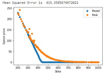
As you can see from the previous graphs, it seems that our model is not doing a very good job in replicating the observed option prices. Is it because of the functional form of the model, or is it just that we did not choose our parameters wisely enough?
3. CEV Model Calibration
Finally, what we are going to do is calibrate this model to the option prices observed in the market. In other words, we are going to minimize the error between our CEV model prices and those prices observed in the market. We are going to optimize by changing only the parameters sigma ($\sigma$) and beta ($\beta$) in our CEV model. Hence, our minimization process will output the parameters sigma and beta that make the error with current market prices lower. This whole process is known as calibration of the model.
- Why do we only focus on these parameters? Remember, risk-neutral valuation.
We will import the minimize module from scipy in order to proceed with the optimization. For now, we will perform a relatively simple minimization with the default procedures in scipy.
We define our error function as the mean squared error (MSE) between model and market prices. This error function is what we will actually minimize.
from scipy.optimize import minimize

def error(params):
    sigma, beta = params
    modelprices = C(Td, test_strikes, sigma, beta)
    realprices = df_call["Last Price"]

    if np.isnan(modelprices).any() or np.isinf(modelprices).any():
        return np.inf

    return mean_squared_error(modelprices, realprices)

bnds = ((0, None), (0, None))
res = minimize(error, (0.65, 1.8), bounds=bnds)
The mean squared error (MSE) should be reduced from the initial scenario.
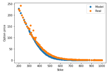
Now, let’s see how the results from the model under the optimized parameters ($\sigma$ and $\beta$) look in a graph versus the real market prices:
modelprices = C(Td, test_strikes, res.x[0], res.x[1])
realprices = df_call["Last Price"]
plt.plot(test_strikes, modelprices, "o", label="Model")
plt.plot(test_strikes, realprices, "o", label="Real")
plt.xlabel("Stike")
plt.ylabel("Option price")
plt.legend()
Conclusion
Congratulations! You’ve successfully implemented and calibrated the CEV model to market data. In the next module, we will continue to work on these ideas, extending the framework to consider the famous stochastic volatility model of Heston.