Bridging the Black-Scholes with Monte Carlo Simulations
Dive in as we journey deeper into the sophisticated world of option pricing. We’ll unravel the enchanting connection between the Black-Scholes analytical model and the ever-versatile Monte Carlo method.
Setting the Stage
Before we start, ensure you have the following libraries:
import matplotlib.pyplot as plt
import numpy as np
import pandas as pd
import numpy.random as npr
from scipy.stats import norm
Delving into Monte Carlo Simulations
You might wonder, “Why bother with Monte Carlo when we have a perfectly good closed-form solution?” This detour becomes invaluable when we delve into realms where analytical solutions don’t exist.
Below are just a few examples of more sophisticated models often don’t have closed-form analytical solutions, and the world of quantitative finance is vast and continually evolving.
Stochastic Volatility Models:
- Heston Model: A model where the volatility itself follows a stochastic process.
- SABR Model: Another stochastic volatility model often used in the interest rate world.
Jump-Diffusion Models:
- Merton’s Jump-Diffusion Model: Incorporates sudden jumps in asset prices in addition to the usual stochastic process.
Local Volatility Models:
- Dupire’s Local Volatility Model: A deterministic function of time and asset price, derived from market prices of European options.
Interest Rate Models:
- Hull-White Model: Used for the dynamics of the short rate (an interest rate applicable to a financial instrument that matures and pays interest in a very short period of time).
Credit Risk Models:
- Cox-Ingersoll-Ross (CIR) Model: Often used to model default probabilities.
Path-dependent options models:
- For exotic options like Asian, barrier, and lookback options, which have payoffs that depend on the entire price path, analytical solutions are often elusive.
Intoruction
The starting point is taking the Brownian motion equation for the underlying stock, $S_t$, in the risk-neutral world:
\[dS = S\,r dt +S\sigma dz\,\]This equation can be discretized using the Euler scheme, leading us to:
\[S_{T} = S_{t} e^{\left(\left(r-\frac{1}{2}\sigma^{2}\right)(T-t) +\sigma \sqrt{T-t}\,z\right)}\,,\]where $z$ is a standard normal random variable.
We can simulate the process above using the Monte Carlo method. As an example, we set $r=0.06$, $\sigma=0.3$, $T-t=1$, $S_t=100$. We make $I=100000$ iterations and choose $M=100$ intervals for the time interval discretization:
Using our handy Python tools, let’s bring this equation to life:
r = 0.06
sigma = 0.3
T = 1.0
S0 = 100
Ite = 100000
M = 100
dt = T / M
S = np.zeros((M + 1, Ite))
S[0] = S0
for t in range(1, M + 1):
    S[t] = S[t - 1] * np.exp(
        (r - 0.5 * sigma**2) * dt + sigma * np.sqrt(dt) * npr.standard_normal(Ite)
    )
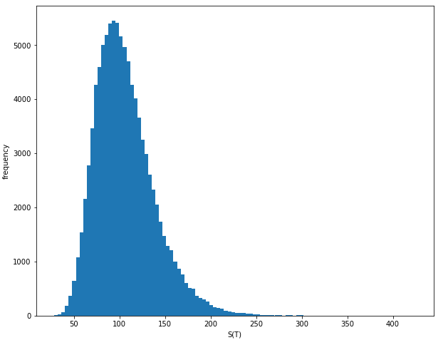
The fruit of our labor should ideally follow a log-normal distribution. Let’s confirm this:
plt.figure(figsize=(10, 8))
plt.hist(S[-1], bins=100)
plt.xlabel("S(T)")
plt.ylabel("frequency")
plt.show()
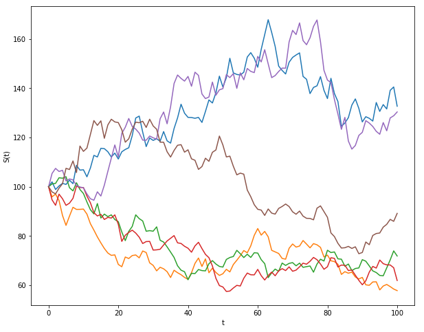
For a more intuitive insight, let’s peek into a few stock price paths:
plt.figure(figsize=(10, 8))
plt.plot(S[:, :6])
plt.xlabel("t")
plt.ylabel("S(t)")
plt.show()
Pricing with Monte Carlo
With our simulated stock prices in hand, let’s calculate the price of a European call option via our Monte Carlo method:
Remember the steps we are doing in the code below:
- Simulate stock price paths according to SDE dynamics.
- Calculate the terminal option payoff for each path.
- Obtain the average expected payoff at maturity, T.
- Discount the average expected payoff to time t.
def bs_call_mc(S, K, r, sigma, T, t, Ite):
data = np.zeros((Ite, 2))
z = np.random.normal(0, 1, [1, Ite])
ST = S * np.exp((T - t) * (r - 0.5 * sigma**2) + sigma * np.sqrt(T - t) * z)
data[:, 1] = ST - K
average = np.sum(np.amax(data, axis=1)) / float(Ite)
return np.exp(-r * (T - t)) * average
Let’s see the pricing power of the previous function with a European call option with the following characteristics:
- $S_0=100$
- $K=95$
- $r=0.06$
- $\sigma = 0.3$
- $T = 1$ year
- $t = 0$ (present day)
- Number of iterations $I=100000$
print("Monte Carlo Price:", bs_call_mc(100, 95, 0.06, 0.3, 1, 0, 100000))
Monte Carlo Price: 17.27360132068741
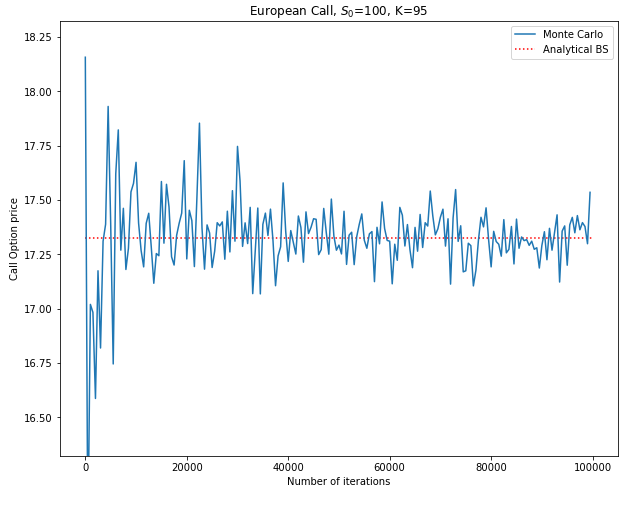
Comparing with Black-Scholes
It’s showdown time! How does our Monte Carlo estimate stack up against the analytical Black-Scholes model?
def bs_call_price(S, r, sigma, t, T, K):
ttm = T - t
if ttm < 0:
return 0.0
elif ttm == 0.0:
return np.maximum(S - K, 0.0)
vol = sigma * np.sqrt(ttm)
d_minus = np.log(S / K) + (r - 0.5 * sigma**2) * ttm
d_minus /= vol
d_plus = d_minus + vol
res = S * norm.cdf(d_plus)
res -= K * np.exp(-r * ttm) * norm.cdf(d_minus)
return res
print("BS Analytical Price:", bs_call_price(100, 0.06, 0.3, 0, 1, 95))
BS Analytical Price: 17.323563283257634
We observe that the Monte Carlo price (17.42) is actually very close to the Black-Scholes analytical price (17.32). As usual, the convergence to the true analytical price will depend on the number of simulations. Thus, once again, we face the trade-off between computational costs and accuracy.
df = pd.DataFrame(columns=["Iter", "BSc"])

for i in range(1, 100000, 500):
    df = df.append(
        {"Iter": i, "BSc": bs_call_mc(100, 95, 0.06, 0.3, 1, 0, i)}, ignore_index=True
    )

plt.figure(figsize=(10, 8))

plt.hlines(
    bs_call_price(100, 0.06, 0.3, 0, 1, 95),
    xmin=0,
    xmax=100000,
    linestyle="dotted",
    colors="red",
    label="Analytical BS",
)
plt.plot(df.set_index("Iter"), lw=1.5, label="Monte Carlo")

plt.title("European Call, $S_0$=100, K=95")
plt.xlabel("Number of iterations")
plt.ylabel("Call Option price")
plt.ylim(
    bs_call_price(100, 0.06, 0.3, 0, 1, 95) - 1,
    bs_call_price(100, 0.06, 0.3, 0, 1, 95) + 1,
)
plt.legend()
plt.show()
Conclusion
Monte Carlo methods, at first glance, might seem superfluous when we have straightforward models like Black-Scholes available. However, its real strength is unveiled in more complex scenarios:
-
Path-dependent options: Monte Carlo is instrumental for options whose payoffs depend on the entire stock price path and not just the value at expiry. Examples include Asian and lookback options.
-
American options: The Black-Scholes model doesn’t provide a solution for these options since they can be exercised at any time before expiration. Monte Carlo simulations, especially when combined with techniques like Least-Squares Monte Carlo (LSMC), offer an avenue for their pricing.
-
Models with jumps: In cases like the Merton jump-diffusion model, where stock prices can make sudden jumps, traditional Black-Scholes falls short. Monte Carlo methods can easily incorporate such complexities.
In essence, Monte Carlo remains a critical tool in the quant’s toolkit. It provides the flexibility and adaptability required to navigate situations where deterministic methods falter. As the world of finance grows more complex, tools that offer such flexibility will only become more valuable.