Ito's Lemma and Black Scholes
Ito’s calculus and the Black-Scholes model are deeply intertwined. Let’s start with an introduction to Ito’s calculus and then explore its connection to the Black-Scholes model.
Ito’s Calculus
Ito’s calculus is a branch of mathematical analysis that deals with stochastic integrals. Its primary developer, Kiyoshi Ito, introduced it to manage integrals where the integrands or integrators are stochastic processes, primarily Brownian motion. The calculus introduces tools to work with integrals of the form:
\[\int_0^t f(t, W_t) dW_t\]Where (W_t) represents a Wiener process or Brownian motion.
Key Features of Ito’s Calculus:
- Ito’s Lemma: Much like the chain rule in classical calculus, Ito’s Lemma provides a way to find the differential of a function of both deterministic and stochastic variables. For a twice-differentiable function (g(t, x)), Ito’s Lemma states:
Given that ((dW_t)^2 = dt), this becomes:
\[dg(t, W_t) = \left( \frac{\partial g}{\partial t} + \frac{1}{2} \frac{\partial^2 g}{\partial x^2} \right) dt + \frac{\partial g}{\partial x} dW_t\]-
Stochastic Integrals: Unlike Riemannian integrals in classical calculus, stochastic integrals, as defined by Ito’s calculus, are non-deterministic since their value depends on the specific realization of the underlying Brownian motion.
-
Quadratic Variation: Ito’s calculus introduces the concept of quadratic variation, crucial for defining and understanding stochastic integrals’ properties. For a Brownian motion (W_t), the quadratic variation over an interval [0, t] is simply (t).
Relation to the Black-Scholes Model:
The Black-Scholes model is a mathematical model used for pricing European-style options. The model’s differential equation assumes that the underlying stock price follows a geometric Brownian motion:
\[dS_t = \mu S_t dt + \sigma S_t dW_t\]Here:
- (S_t) is the stock price at time (t)
- (\mu) is the expected return of the stock
- (\sigma) is the stock’s volatility
- (dW_t) is an increment of a Wiener process or Brownian motion.
The Black-Scholes model emerges naturally when attempting to derive a no-arbitrage price for a European option, given the assumption of log-normally distributed returns. The derivation of the Black-Scholes partial differential equation relies heavily on Ito’s Lemma to handle the stochastic differential term (\sigma S_t dW_t).
In essence, the relationship between Ito’s calculus and the Black-Scholes model can be summarized as follows:
- The Black-Scholes model assumes stock prices follow a stochastic process, particularly geometric Brownian motion.
- Ito’s calculus provides the tools necessary to work with such stochastic processes.
- The derivation of the Black-Scholes equation uses Ito’s Lemma to transition from the stochastic differential equation governing stock price movement to the partial differential equation that the option price satisfies.
BS in Practice
A foundational assumption of the Black-Scholes model is the log-normal distribution of stock prices. This assertion has both empirical and theoretical underpinnings.
To investigate this empirically, we’ll pull some historical stock data:
import matplotlib.pyplot as plt
import numpy as np
from scipy.stats import lognorm, norm
import yfinance as yf

stocks = yf.Tickers("AAPL AMZN")
hist = stocks.history(start="2000-01-01", end="2021-03-31")
prices = hist["Close"]

plt.hist(prices["AMZN"], bins=75, label="AMZN Stock Prices")
plt.legend()
plt.show()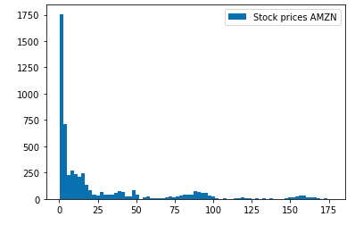
Observe the shape it forms—a hint of log-normality. To further substantiate this:
s = np.log(r)
plt.hist(s, label="Transformed Normal Density")
plt.legend()
plt.show()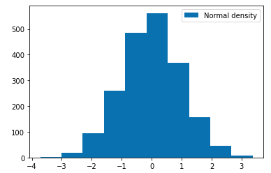
The Black-Scholes Model in Action: Pricing a Call Option
With a grasp on stock price distribution, we transition into the heart of the Black-Scholes model.
Let’s start by building a function (bs_call_price) that returns the value of a call option under the Black-Scholes model. Remember:
$c = S_0 \mathcal{N}(d_1) - K e^{-rT}\mathcal{N}(d_2) $
def bs_call_price(S, r, sigma, t, T, K):
    ttm = T - t

    if ttm < 0:
        return 0.0
    elif ttm == 0.0:
        return np.maximum(S - K, 0.0)

    vol = sigma * np.sqrt(ttm)

    d_minus = np.log(S / K) + (r - 0.5 * sigma**2) * ttm
    d_minus /= vol

    d_plus = d_minus + vol

    res = S * norm.cdf(d_plus)
    res -= K * np.exp(-r * ttm) * norm.cdf(d_minus)

return resprint(bs_call_price(100.0, 0.0, 0.2, 0, 2.0, 105.0))
9.19735064929452The Greeks: Sensitivities in Option Pricing
Option pricing doesn’t exist in isolation. It’s susceptible to various market factors, and this is where ‘The Greeks’ play a pivotal role:
- Delta: Evaluates the option price sensitivity concerning the underlying asset’s price.
- Gamma: Delves deeper, examining Delta’s sensitivity to the underlying price.
- Vega: Probes into the option price’s reaction to volatility.
- Theta: Chronicles the effects of time decay on option price.
- Rho: Investigates the influence of interest rates on the option price.
The computation:
import numpy as np
import scipy.stats as ss

# Data for input in Black-Scholes formula:

T = 2.0  # supposed in years. It is not the maturity, but the time to maturity
S = 100.0
K = 105.0
r = 0
vol = 0.20  # supposing it is annual
option_type = "C"  # for the put insert 'P'
# dividend yield assumed to be 0

# Compute d1 and d2
d1 = (np.log(S / K) + (r + 0.5 * vol**2) * T) / (vol * np.sqrt(T))
d2 = d1 - vol * np.sqrt(T)

if option_type in ["C", "P"]:
    if option_type in ["C"]:
        Opt_Price = S * ss.norm.cdf(d1) - K * np.exp(-r * T) * ss.norm.cdf(d2)
        Delta = ss.norm.cdf(d1)
        Gamma = ss.norm.pdf(d1) / (S * vol * np.sqrt(T))
        Vega = S * ss.norm.pdf(d1) * np.sqrt(T)
        Theta = -(S * ss.norm.pdf(d1) * vol) / (2 * np.sqrt(T)) - r * K * np.exp(
            -r * T
        ) * ss.norm.cdf(d2)
        Rho = K * T * np.exp(-r * T) * ss.norm.cdf(d2)
    else:
        Opt_Price = K * np.exp(-r * T) * ss.norm.cdf(-d2) - S * ss.norm.cdf(-d1)
        Delta = -ss.norm.cdf(-d1)
        Gamma = ss.norm.pdf(d1) / (S * vol * np.sqrt(T))
        Vega = S * ss.norm.pdf(d1) * np.sqrt(T)
        Theta = -(S * ss.norm.pdf(d1) * vol) / (2 * np.sqrt(T)) + r * K * np.exp(
            -r * T
        ) * ss.norm.cdf(-d2)
        Rho = -K * T * np.exp(-r * T) * ss.norm.cdf(-d2)
else:
    Opt_Price = "Error: option type incorrect. Choose P for a put option or C for a call option."

print("Option price = {}".format(Opt_Price))
print("Delta = {}".format(Delta))
print("Gamma = {}".format(Gamma))
print("Vega = {}".format(Vega))
print("Theta = {}".format(Theta))
print("Rho = {}".format(Rho))

Option price = 9.197350649294513
Delta = 0.4876036978454982
Gamma = 0.014097929791127266
Vega = 56.39171916450907
Theta = -2.819585958225453
Rho = 79.1260382705106
The Black-Scholes model, with its inherent beauty and robustness, remains a cornerstone in quantitative finance. Our exploration today, through stock price distribution to the intricacies of option pricing and sensitivities, underscores its undiminished relevance.
As we conclude, remember that the journey of understanding doesn’t end here. The world of quantitative finance is vast and ever-evolving, and the Black-Scholes model is but one star in this expansive universe.