Intro to Monte Carlo methods
History lesson
The Monte Carlo method, a groundbreaking statistical technique, was named after the famous Monte Carlo casino in Monaco, not because it was created there, but due to the method’s use of randomness and chance, reminiscent of gambling. The method was developed during the 1940s by physicists Stanislaw Ulam and John von Neumann while they were working on nuclear weapons projects at the Los Alamos National Laboratory in the United States.
The story goes that Ulam was recovering from an illness and was playing a lot of solitaire. He became interested in calculating the chances of winning a particular solitaire game but found that calculating it deterministically would be incredibly complex. Instead, he realized that he could get a reasonable estimate by simply playing the game many times (or having a computer play it) and observing the fraction of games he won.
Ulam discussed this ‘statistical sampling’ technique with John von Neumann, and the two of them developed it into a general method for approximating complex mathematical calculations using random sampling — essentially, using randomness to solve problems that might be deterministic in principle, but are too complex to solve in a deterministic manner.
von Neumann realized the potential of this method in the context of the ongoing work at Los Alamos, and it soon became an essential tool for the Manhattan Project, allowing the scientists to model the random behavior of particles to understand complex physical systems.
That’s why it is called the Monte Carlo method: because it employs randomness and probability, much like the games of chance played in the famous casino.
Introduction
Monte Carlo methods, a powerful technique that plays a critical role in modern quantitative finance. We’ll begin with a basic introduction, aiming to build a solid foundation that will be valuable when tackling more complex problems later in the series.
At its core, the Monte Carlo method is a statistical technique that allows us to approximate complex mathematical problems using random sampling. Here’s the basic idea:
- Simulate a large number of random samples from the same distribution as our underlying process.
- Calculate the option payoff for these simulated values and discount them.
- Take the average of these discounted payoffs. As the number of simulations increases, this average converges to the option’s true value.
Now let’s start by importing the numpy library:
import numpy as npWe will develop a function, call_option_mc, to illustrate the power of Monte Carlo methods:
def call_option_mc(S_ini, K, T, r, sigma, N, M):
    dt = T / N  # Define time step
    u = np.exp(sigma * np.sqrt(dt))  # Define u
    d = np.exp(-sigma * np.sqrt(dt))  # Define d
    p = (np.exp(r * dt) - d) / (u - d)  # risk neutral probs
    C = np.zeros([M])  # call prices
    S = np.zeros([M, N + 1])  # underlying price
    S[:, 0] = S_ini

    for j in range(0, M):
        random = np.random.binomial(
            1, p, N + 1
        )  # We sample random realizations for the paths of the tree under a binomial distribution
        for i in range(1, N + 1):
            if random[i] == 1:
                S[j, i] = S[j, i - 1] * u
            else:
                S[j, i] = S[j, i - 1] * d

        C[j] = np.exp(-r * T) * max(S[j, N] - K, 0)

    return S, C
European Call Option Payoff (Monte Carlo)
In this example, we’re focusing on a European call option. We have already defined a function call_option_mc that prices this option using Monte Carlo simulations.
Given the option characteristics:
S=100
K=90
T=1
r=0%
σ=0.3
Let’s see how our Monte Carlo algorithm performs:
S, C = call_option_mc(
    100, 90, 1, 0, 0.3, 2500, 15000
)  # Prices 15000 different simulations

print(np.mean(C))
16.99442814458002
As you can see, the value is pretty close to the one we got from the workout earlier on the full binomial model of $17.01.
Asian Option Payoff (Monte Carlo)
Unlike European or American options, Asian options have a payoff that depends on the average price of the underlying asset over a certain period, not just the price at a specific point in time.
For our Asian option, we’ll use the same parameters we used for the European option and will build a function asian_option_mc:
def asian_option_mc(S_ini, K, T, r, sigma, N, M):
    dt = T / N  # Define time step
    u = np.exp(sigma * np.sqrt(dt))  # Define u
    d = np.exp(-sigma * np.sqrt(dt))  # Define d
    p = (np.exp(r * dt) - d) / (u - d)  # risk neutral probs
    Asian = np.zeros([M])  # Asian prices
    S = np.zeros([M, N + 1])  # underlying price
    S[:, 0] = S_ini

    for j in range(0, M):
        random = np.random.binomial(1, p, N + 1)
        Total = S_ini
        for i in range(1, N + 1):
            if random[i] == 1:
                S[j, i] = S[j, i - 1] * u
                Total = Total + S[j, i]
            else:
                S[j, i] = S[j, i - 1] * d
                Total = Total + S[j, i]

        Asian[j] = np.exp(-r * T) * max(Total / (N + 1) - K, 0)

return S, AsianS, Asian = asian_option_mc(100, 90, 1, 0, 0.3, 2500, 10000)And average them to get a final estimate:
print(np.mean(Asian))
12.342288405943835
Let’s also study the convergence of the methods in a similar fashion as before:
M = np.arange(1000, 16000, 1000)
asian_price = []
for i in range(len(M)):
S, Asian = asian_option_mc(100, 90, 1, 0, 0.3, 2500, M[i])
asian_price.append(np.mean(Asian))
import matplotlib.pyplot as plt
plt.plot(M, asian_price)
plt.ylim([10, 15])
plt.title("MC Estimates for different # simulations")
plt.xlabel("Number of Simulations")
plt.ylabel("Asian Call Option Price")
plt.grid(True)
plt.show()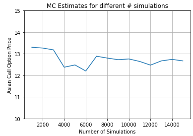
Conclusion
By now, you’ve witnessed firsthand how Monte Carlo methods can be a formidable tool when pricing complex derivatives. This technique is especially useful when calculating all the potential payoffs of an option is impractical due to computational constraints.
While this post introduces Monte Carlo from an informal perspective, we aimed to simplify your understanding of it. We plan to explore this topic in further depth in future posts.