Introducing Delta
Now we are going to dive deeper into some fundamental concepts of option pricing, specifically in a binomial tree. We’ll then introduce the concept of delta hedging, a strategy used to hedge against price movements in the underlying asset.
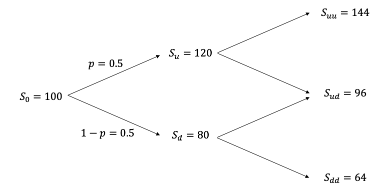
To set the scene, let’s think of a situation where the underlying stock price distribution is captured in a graph. This is based on a risk-free rate r=0, and we’re working on pricing a call option with a strike price K=90.
We’ll start with importing necessary Python libraries:
import numpy as npDelta Hedging in the Binomial Tree
Let’s dive right into the code that computes various aspects of our European call option using the binomial tree approach:
def call_option_delta(S_ini, K, T, r, u, d, N):
    dt = T / N  # Define time step
    p = (np.exp(r * dt) - d) / (u - d)  # risk neutral probs
    C = np.zeros([N + 1, N + 1])  # call prices
    S = np.zeros([N + 1, N + 1])  # underlying price
    Delta = np.zeros([N, N])  # delta
    for i in range(0, N + 1):
        C[N, i] = max(S_ini * (u ** (i)) * (d ** (N - i)) - K, 0)
        S[N, i] = S_ini * (u ** (i)) * (d ** (N - i))
    for j in range(N - 1, -1, -1):
        for i in range(0, j + 1):
            C[j, i] = np.exp(-r * dt) * (p * C[j + 1, i + 1] + (1 - p) * C[j + 1, i])
            S[j, i] = S_ini * (u ** (i)) * (d ** (j - i))
            Delta[j, i] = (C[j + 1, i + 1] - C[j + 1, i]) / (
                S[j + 1, i + 1] - S[j + 1, i]
            )
    return C[0, 0], C, S, Delta
This function gives us the underlying asset’s evolution, the call option’s price at each tree node, and the delta at each node.
To better understand this function, consider the following example:
price, call, S, delta = call_option_delta(100, 90, 15, 0, 1.2, 0.8, 15)
print("Underlying: \n", S)
print("Call Price: \n", call)
print("Delta: \n", delta)
This outputs the underlying asset price, call price, and delta for all nodes.
To hedge the sale of the call option (from a bank’s perspective), one would:
Buy 0.675 shares at t=0. At t=1, hold 0.1875 shares if the price goes down or 1 share if the price increases.
By following this strategy, the resulting total cost would be $16.5, which matches the call price.
Generalization to Any N
Once we understand the basic example, generalizing the tree and hedging strategy for any number of time steps becomes straightforward.
#### Convergence How does the option price change with different time steps, N? Let’s visualize:
price_array = []
for N in [1, 10, 100, 200, 300, 400, 500, 600, 700, 800, 900, 1000, 1500, 2000, 2500]:
    price, call, S, delta = call_option_delta(100, 90, 1, 0, 1.2, 0.8, N)
    price_array.append(price)
    print("With N = {:3d}, the price is {:.2f}".format(N, price))
With N = 1, the price is 15.00
With N = 10, the price is 29.38
With N = 100, the price is 70.32
With N = 200, the price is 85.40
With N = 300, the price is 92.33
With N = 400, the price is 95.84
With N = 500, the price is 97.70
With N = 600, the price is 98.71
With N = 700, the price is 99.27
With N = 800, the price is 99.58
With N = 900, the price is 99.76
With N = 1000, the price is 99.86
With N = 1500, the price is 99.99
With N = 2000, the price is 100.00
With N = 2500, the price is 100.00This code iterates through different values of N, and for each, computes the price of the option.
In a more visual form:
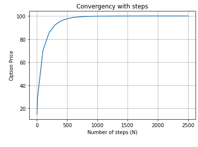
This visualization prompts us to ponder: Why does the price behave in this particular manner as we increase the number of steps?
The more steps we use, the finer the granularity of our simulation, meaning we capture more possible price paths of the underlying.
Discreteness vs. Continuity: A binomial model is inherently discrete, meaning it breaks down the time to expiration into small intervals and considers the price movement of the underlying asset at each interval. As we increase the number of steps, this model approximates a continuous model, which is often more accurate and reflective of the real world. The Black-Scholes model for option pricing, for instance, is a continuous model.
Law of Large Numbers: As the number of steps increases, we are effectively taking more samples of possible price paths. This allows our model to converge to a more ‘expected’ or ‘average’ result due to the law of large numbers, which states that as the number of trials in a random experiment increases, the average of the results should get closer to the expected value.
Model Convergence: As the number of steps N approaches infinity, the binomial model price will converge to the Black-Scholes model price. This is because the binomial model becomes a closer approximation of the continuous stochastic differential equation that underpins the Black-Scholes model.
We’ve navigated through the intricacies of option pricing in the binomial model and seen the effects of varying the number of steps in our model. This exercise underscores the importance of understanding delta hedging and the underlying assumptions in our model. As we’ve seen, the choice of parameters can lead to different pricing results, which has significant implications for hedging strategies and risk management in finance.